Psycho-physiological interaction (PPI)
PPI (psychophysiological interactions) is a method for finding out whether the correlation in activity between two distant brain areas is different in different psychological contexts – in other words whether there is an interaction between the psychological state and the functional coupling between two brain areas.
Most of the content of this web page, together with some material relating PPI to resting state analysis, has been published as a Tools of the Trade article in SCAN:
Jill X. O’Reilly, Mark W. Woolrich, Timothy E.J. Behrens, Stephen M. Smith, Heidi Johansen-Berg, Tools of the trade: psychophysiological interactions and functional connectivity, Social Cognitive and Affective Neuroscience, Volume 7, Issue 5, June 2012, Pages 604–609, https://doi.org/10.1093/scan/nss055
PPI was originally implemented in SPM. You can read the original paper in NeuroImage:
Psychophysiological and modulatory interactions in neuroimaging. Friston KJ, Buechel C, Fink GR, Morris J, Rolls E, Dolan RJ. Neuroimage. 1997 Oct;6(3):218-29.
Some presentation slicdes given by Jill O'Reilly can be downloaded here.
Overview
A hypothetical example... Say we had run an experiment where participants have to navigate through a virtual reality maze (compared to a control condition where they travel passively through a maze), and we found that prefrontal cortex and hippocampus were active for navigation – that is, in the GLM contrast [navigation–passive travel]. We might come up with (at least) two possible explanations:
- the prefrontal cortex and hippocampus were both independently active in the navigation condition (say, because navigation requires planning which involves the PFC, and because navigation requires spatial information which is stored in the hippocampus).
- The PFC and HPC work together interactively in navigation – perhaps some ‘top down’ signal from the PFC causes retrieval of information in the hippocampus, which is then passed back to the prefrontal cortex.
A PPI analysis could help us distinguish between these two hypotheses by telling us whether the correlation in activity between the two areas, rather than activity itself, increased in the navigation task.
Correlations
How do we go about looking for areas which interact with the hippocampus? The first principle underlying PPI is that if two areas are interacting, the level of activity in those areas will correlate over time – in other words if activity in the two areas increases and decreases ‘in synch’ this suggests that there is a functional association between them.
So we have a basic strategy: we can extract the time-course from some representative voxel in the hippocampus and run a GLM using this hippocampal activity time-course the explanatory variable. Areas with a high Z-score are the ones which vary their activity ‘in synch’ with the hippocampus.
Psychophysiological interactions
The second principle underlying PPI analysis is that the interactions between areas may change in different psychological contexts, and this will be reflected in a change in correlation between the time-courses of those areas. Say, for example, that when people navigate around a maze, the hippocampus and the prefrontal cortex interact as people use spatial information (represented in the hippocampus) to plan their route (as planning requires PFC) – but in the passive travel condition these two regions do not interact. Then we would expect the correlation in activity between the two regions to be higher during the navigation condition than during the passive travel condition. In a psychophysiological interactions analysis, we particularly look for areas which have a higher correlation with the time-course in the seed region in one psychological context (task block) than another.
To put this another way, it is quite likely that some brain regions will share a time-course of activity with your seed region but that this correlation has nothing to do with your experiment per se – for example, regions which are anatomically connected, regions which share neuro-modulatory influences and regions which share sensory input will all have correlated time-courses regardless of what experiment you are doing. In PPI we are only interested in relationships which change with the task in your experiment, for example areas which interact during navigation but not during passive travel.
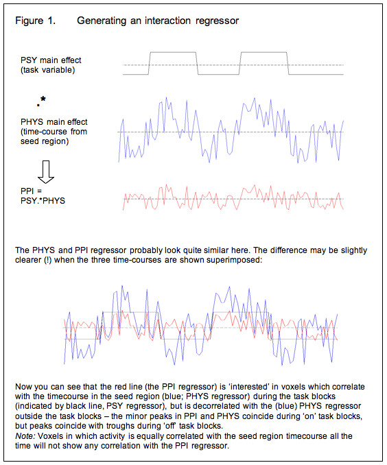
So now we modify the basic strategy: Instead of using the time-course of the seed region as an explanatory variable in the GLM, we generate an ‘interaction regressor’ and use this instead. Generally speaking, the interaction regressor will be the (demeaned) scalar product of the (demeaned) task time-course and the (demeaned) physiological time-course (time-course of activity in the seed region) although the generation of the interaction term is discussed in more detail below. Or, in other words, voxels in which the interaction term is a good description of activity are those in which the seed region’s time course has a stronger effect during the task blocks of interest than it does the rest of the time.
Covariates of no interest
So now we have a GLM in which the explanatory variable is the interaction term described above. This tells us which regions are more correlated with the seed region during the task of interest than at other times. But there is a problem with this approach: because we generated the interaction term as the product of the psychological and physiological ‘main effects’ variables, regions in which those main effects account for a lot of the variance will show up as being related to the interaction term. To spell this out:
- We selected the (seed) region of interest on the basis that it was active in a certain contrast (in our example, navigation-passive travel), and therefore we are pretty much certain to see a correlation with all the other areas which were active in that contrast in our original GLM (because these also increase in activity during the navigation blocks). In other words, we will observe correlations which are driven by a shared task input, which is exactly what we already knew from the GLM analysis.
- Voxels which have a similar time-course to the seed region, even if this is not task related, will have a positive correlation with the interaction term, although not as strong as those in which the correlation is task related.
To avoid these issues, we modify our strategy again and include the psychological and physiological time-courses from which we derived the interaction term in the GLM as covariates of no interest. This means that variance associated with the interaction term is only that over and above what is accounted for by the main effects of task and physiological correlation. This is the final PPI model.
Between subjects designs: an alternative approach
A few studies (listed below) have used PPI-like analyses in between-subjects designs, treating subject group as the 'psychological' variable. For example, Heinz et al (2005) investigated differences in coupling of the amygdala with the rest of the brain between people with different genotypes for the serotonin transporter gene SLC6A4. Because they were interested in a functional coupling which was assumed to be determined by genotype, which does not change over the course of the scanning session they simply extracted the time-course of activity from an ROI in the amygdala and entered this into the GLM for each subject. The resulting maps simply showed which regions correlated in time-course with the amygdala in the three genetic groups.
Because, in this case, the authors used the whole time-series from their scanning session to compare between groups, there was no task regressor (PSY) to include in the model – effectively the PSY variable was genotype. Because of this, the ‘PPI’ regressor was exactly the same as the time-course of the amygdala ROI (PHYS) in each subject, so that was not included either – so only the PPI regressor was entered into the GLM for each individual. Clearly, this gets around the problem of correlated regressors described above.
The same approach has been used to compare patients with Turner syndrome to normal controls (Skuse et al 2005), to compare schizophrenic patients to healthy controls (Boksman et al 2005). By the same justification, we could use this approach to look at changes in functional connectivity following TMS or TDCS, or between patient and normal groups.
However, it seems to me that there is a problem with this approach. As long as people are doing a task during the scan sessions and the groups show different activation patterns during this task, the ‘PPI’ can be driven by a main effect of task. For example, in Heinz (2005), the non-carriers of the SLC6A4 allele showed higher amygdala activation in response to the aversive stimuli than to the neutral stimuli. Because the task contrast was not modelled in the ‘PPI’ analysis, any areas with the same task driven effect would show up as having higher ‘functional connectivity’ in the no-carrier group, because only the non-carriers showed an effect of task.
A way around this problem is to include only those portions of the time-course which correspond to the task blocks of interest, and to de-mean the seed time-course within these blocks to ‘partial out’ the main effect of task. Bear in mind that this approach would not detect a ‘main effect’ of task; the assumption is that since the task is the same, we are only interested in the between sessions effect.
Papers using some kind of between-subjects approach: - Heinz A, Braus DF, Smolka MN, Wrase J, Puls I, Hermann D, Klein S, Grüsser SM, Flor H, Schumann G, Mann K & Büchel C (2004) Amygdala-prefrontal coupling depends on a genetic variation of the serotonin transporter Nature Neuroscience 8, 20 – 21
Boksman K, Theberge J, Williamson P, Drost DJ, Malla A, Densmore M, Takhar J, Pavlosky W, Menon RS, Neufeld RW. (2005) A 4.0-T fMRI study of brain connectivity during word fluency in first-episode schizophrenia. Schizophr Res. 15:247-63
Skuse DH, Morris JS, Dolan RJ. (2005) Functional dissociation of amygdala-modulated arousal and cognitive appraisal, in Turner syndrome. Brain. 128:2084-96
Bingel U, Lorenz J, Schoell E, Weiller C, Buchel C. (2006) Mechanisms of placebo analgesia: rACC recruitment of a subcortical antinociceptive network. Pain 120:8-15
TMS-Induced changes to a physiological network
A PPI-like approach can be used to look at how functional networks reorganise when one area in the network is ‘damaged’ by TMS. This method was used by:
O’Shea J, Johansen-Berg H, Trief D, Goebel S and Rushworth MFS (2007). Functionally specific reorganisation in human premotor cortex Neuron 54: 479-490
They looked at action selection, which engages the dorsal pre-motor cortex, particularly the dominant left PMd (L PMd). They compared activation in an action selection task with a simple motor control task, before and after disrupting the L PMd with a 15 min 1 Hz TMS train – a type of stimulation which causes local suppression of activity lasting several minutes.
As expected, the TMS had the effect of suppressing activity in L PMd. They then asked: can suppression of activity in L PMd account for changes in activity in other brain areas (which had not been directly affected by TMS)? To do this, they generated ‘PPI’ regressors with the following properties: during the selection task blocks, the PPI regressor was the same as the (demeaned) time-course of activity in L PMd; during the control task blocks the PPI regressor was the negative (x -1) time-course of L PMd; and outside the task blocks, it was zero. In other words, the PPI regressor reflected the activity of L PMd in the task contrast selection-control. They then compared the ‘PPI’ effects before and after TMS, to see how the changed response of L PMd to the task fed into other brain areas.
Note that this approach is rather different from the (typical) PPI analyses described above, which look for effects over and above the main effect of psychological task. Here, the main effect of task was not removed from the data in any way, but was assumed to be the same between sessions, whilst the only difference between sessions was how the main effect of task was mediated by activity in L PMd, which was suppressed after TMS. Thus this approach answers a different question from a typical PPI analysis.
How to run a PPI analysis in Feat
1. Make some decisions
Because you start by choosing and ROI and task contrast, PPI is heavily hypothesis driven. If you don’t have a clear hypothesis about functional connectivity, you might consider using a model-free approach like MELODIC, which also gives you ‘network’ information of a different kind. On the other hand, you can also try running lots of different PPIs with different seed regions until you find something interesting… .
Choose your ROI
For a PPI analysis, you must select a seed Region of Interest (ROI) – the point of the analysis is to look for areas which ‘interact’ with this seed region.
There are several types of ROI you might go for:
-
An anatomical region of interest. For example, you might have an a priori hypothesis about the functional connectivity, in your task, of the hippocampus, or the putamen, or some other region which you can define from a structural scan.
-
An ROI based on functional activations from your initial GLM (Feat) analysis. For example, you might find a few blobs associated with your task of interest, and you hypothesis that these blobs can be grouped into a couple of separate networks. Maybe you were doing a memory task, and it activated the hippocampus. You have some idea what the hippocampus is doing, so now you want to know which areas have increased functional connectivity with it during your task, and which areas are involved, but not interacting with the hippocampus.
-
An ROI based on a local maximum in one of your MELODIC components. For example, say you analyzed your data with group-MELODIC and you found the two biggest components were, say, an attentional (dorsal, frontal-parietal) network and a memory network (say, prefrontal and medial temporal areas). And say your experiment looked at how your memories can bias your attention, comparing trials with familiar stimuli and novel stimuli. Then the attention and memory networks might describe the two major cognitive components of your whole dataset (all trials together) - but for you the critical point of interest is whether there is more interaction between networks in your attention-from-memory task. You can pick a blob from one of your melodic components, which you think might be the 'linking' node, and use it as the seed for a PPI, which tells you about task-specific interactions. Note that MELODIC blobs may be more likely to be 'good' seeds for your PPI analysis than GLM/Feat blobs, because MELODIC is a more network-oriented type of analysis.
Choose your task contrast
PPI analysis always looks for voxels with increased functional connectivity to your seed ROI in one condition compared to another. Usually, the contrast will be between conditions within a single scanning session, and you need to decide whether this will be a contrast of one condition vs everything else (a 1 0 contrast) or a contrast between two conditions (a 1 -1 contrast). More details about this are in the FAQ.
However, you may also be interested in comparing between scanning sessions, for example before and after an intervention, such as a drug or brain stimulation - or even betweens groups (e.g. patients vs. controls). A discussion of between-subjects designs can be found above.
2. Prepare your regressors
You need to extract the timecourse from the seed ROI and put it into a format which Feat can read, before using Feat to make your PPI regressor.
Make masks for the seed ROI
You need to make a mask for your seed region in each individual subject’s functional native space (that is, the space of the fMRI image you want to analyse).
Anatomical region of interest
Your options are:
- Draw a mask on individuals’ structural scans with FSLeyes
- Draw a mask on the standard brain and transforming it into individual space using FLIRT or FNIRT
- Use an automated segmentation tool eg FIRST.
Functional region of interest
Your options are:
- On your group Feat results/ MELODIC component, draw a region of interest over the blob you are interested in. Transform this into the functional space of each individual using FLIRT or FNIRT. Check, for each individual, that your ROI is a sensible size and is contained within the brain and within the anatomical region of interest (if your ROI is near the surface and ends up lapping over the edge of the brain in some subjects, your timecourse data will be very noisy, so you really do need to check).
- Go to each individual subject's Feat results and pick the peak voxel in the region of interest. Draw a small mask surrounding this peak voxel.
This may be a more successful strategy when the functional regions are anatomically heterogeneous but functionally well defined, e.g. in the parietal cortex.
Size of ROIs
If you are defining ROIs individually (as in the second functional-ROI case, or some of the anatomical cases) you analysis will likely work better (have higher signal-to-noise) if you keep the ROI small. This is because you are only taking one measurement from the whole ROI – so by enlarging the ROI to include voxels with a weaker effect you are actually ‘watering down’ the signal.
On the other hand, if you are using a standard-space mask (as in the first functional-ROI strategy), you will want to make sure your ROI is large enough to capture the individual activation peak for each subject, despite inter-individual variations.
Extract the time-course of the seed ROI
Do this for each subject separately, using the fslmeants command.
You should use the filtered_func_data from your initial analysis to extract the timecourse from - not the raw data as this will be noisy.
fslmeants -i filtered_func.nii.gz -o my_timecourse.txt -m your_roi_mask.nii.gz
The output is a column vector giving a value of raw signal at each time-point; there is one time-point per volume. The time-course is saved under a filename specified by you, for use later on.
3. Set up your Feat design
Start FEAT and load your data and set up your pre-processing as normal. If you are using the filtered_func_data from your GLM analysis as input, remember not to re-do any pre-processing steps such as BET, deleting volumes, or filtering.
In the stats tab
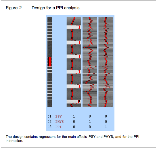
You will need the following regressors:
-
EV1 is your psychological regressor (PSY). This will simply be your task regressor, convolved with an HRF.
-
EV2 is your physiological regressor (PHYS). This will be the time-course of your seed ROI:
- Basic shape is ‘custom (1 entry per volume)’ and the input file is the time-course from the seed region, which you generated earlier with fslmeants.
- Set convolution to none because this is BOLD data and has already been convolved by the brain!
- Switch off temporal derivative and temporal filtering
-
EV3 is PPI, which you generate here in the Feat GUI:
- Basic shape is interaction
- Between EVs: select EV1 and EV2
- Make zero - these drop down boxes give you the choice of Min, Centre and Mean (read more about the zero-ing options here. You should choose:
- centre for your task (PSY) EV, and
-
mean for your ROI timecourse (PHYS) EV.
-
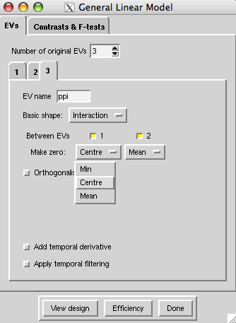
Orthogonalise: You should probably not do this. If in doubt, have a look at the notes on orthogonalizing in the FEAT guide. Effectively, orthogonalizing means that the stats for the EV you orthogonalize with respect to (not the EV where you click the 'orthogonalize' button) change. Why? Because in the GLM, if some activity in your voxel is correlated with BOTH EVs A and B, is is not assigned to either. Now, If A and B are partially correlated (eg if they are your PSY and PPI) then some activity in some voxels may be correlated with the correlated part of A and B. This activity is therefore assigned to neither A nor B. Orthogonalizing B with respect to A changes regressor B, to remove the part which was correlated with A. This means that the activity which was correlated with both A and B, which was previously not modelled, is now only correlated with A - so the estimate for EV A changes. The esitmate for EV B stays the same, because you have only taken away the part of that EV which was correlated with A, and therefore didn't get any activity assigned to it anyway. Now, in Feat you always orthogonalize the later-created EV w.r.t. the earlier-created one, and the PPI EV will necessarily be created after the task EV- So if you were to orthogonalise your PPI EV with respect to your task EV, the effect of orthogonalizing would be on the results for the main effect of task, not on the PPI effect. - Switch off temporal derivative and temporal filtering
Other task regressors: As well as the three EVs described here, you should include all the task EVs you included in your original model, in the setup for the PPI analysis. So your setup should look like the setup for your original (standard) Feat analysis, but with the physiological and PPI regressors added. The model describes the data better if all task EVs are included.
This completes the set-up for the first-level analysis. You can then compare between groups at the second level as normal.
Zeroing options in PPI
When you create a regressor of type 'interaction' in the stats tab of the Feat gui, you to select from a drop down list called 'zero' for each regressor which is going into your PPI.
1. Min
Zero min makes the minimum value of the regressor zero.
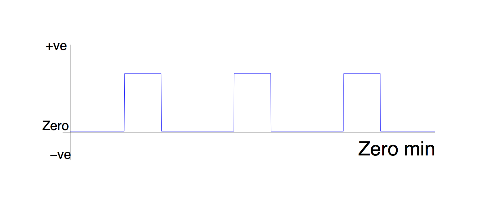
If you do this to a task (PSY) EV, you will essentially be setting the value of the PSY part of the PPI to zero during your rest blocks. Since multiplying any number by zero gives zero, this means that your PPI regressor will be a flat line in the rest blocks. In other words, your PPI regressor looks like the timecourse of your seed ROI during the task, and zero otherwise.
This type of PPI regressor is looking for voxels which are correlated with the seed ROI during the task - but they don't actually have to be more correlated during the task than elsewhere.
Think about it this way: imagine some voxel was always correlated with your seed region. If you de-min the PSY part of your PPI, and create a PPI regressor like the one above, then that PPI regressor will still 'pick up' that voxel - even though the correlation is not task-specific.
When would you use this option for the PSY component? In the case that you are doing a between-subjects or between-sessions design, and you want to 'partial out' the any changes in the main effect of subjects/sessions on your task. This is discussed further here.
When would you use this option for the PHYS component? Don't.
2. Centre
Zero centering sets zero to be halfway between the highest and lowest points of the regressor.
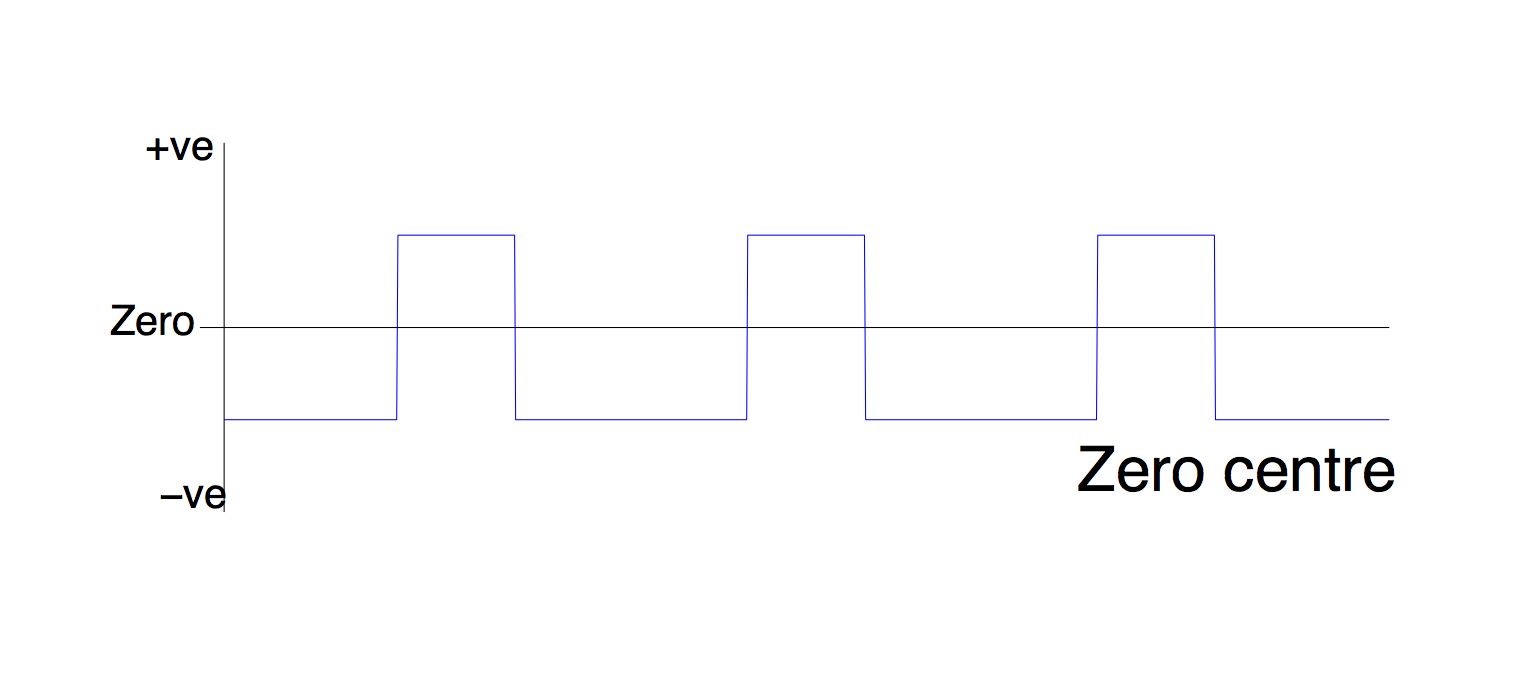
This means that the 'on' and 'off' periods of your design are treated equally even if they have different durations - in effect it created a 1, -1 contrast between the 'on' and 'off' blocks of your task.
Why is this different from de-meaning (option 3)? Imagine that you have 'on' and 'off' blocks of un-equal length, say the 'off' blocks are twice as long, and you de-mean this (literally, subtract the mean, which is nearer to the height of the 'off' blocks, since these make up more of the time). The resulting regressor will have higher blocks in the on period than the off period - twice as high, in fact. Now you multiply this with your ROI timecourse to get a PPI regressor. In other words, you are multiplying the timecourse by -1 during the off blocks, and +2 during the on blocks.
This regressor is looking for voxels which are twice as correlated with your seed ROI in the on block, as in the off block. This means you need double the effect to get a significant result - obviously increasing the chance of a false negative.
What you really want is to multiply the ROI timecourse by -1 diring the off blocks and +1 during the on blocks. Using the zero-centre option does this for you.
When would you use this option for the PSY component? Any time you are doing a within-subjects design
When would you use this option for the PHYS component? Don't.
3. Mean
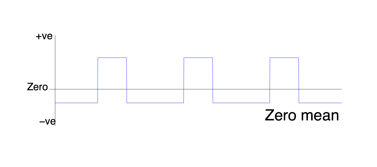
This option literally subtracts the mean from the regressor. You want to do this for your ROI timecourse (PHYS regressor).
When would you use this option for the PSY component? Don't. Although if you have used this instead of zero-centring in a previous analysis, it can only have increased the chance of a false negative.
When would you use this option for the PHYS component? Always.
Caveats
This section highlights some potential issues with PPI. However, note that lots of papers using PPI have been published, and there are always issues with every method, so you shouldn’t get too bogged down with these worries. In fact, if you are the bogging-down-in-worry type, better stop reading now.
What exactly does PPI model?
A PPI effect is a task-specific change in correlation between areas, which cannot be explained simply by a shared effect of task. What neural processes could generate such a correlation?
One answer is probably unmodelled task related variance For example, say that in the hypothetical maze-navigation experiment above, we have modelled navigation using a block design (navigate/passive travel/rest modelled as boxcars). What if PFC and HPC (independently) only really get involved in navigation when you turn a corner? Then the true shape of the psychological variable is rather more phasic than the boxcar we modelled, and thus there is unmodelled task-related variance shared between the PFC and HPC which could be driving both areas. This would lead to a spurious PPI.
A second type of unmodelled variance would be learning effects – for example in a sequence-tapping task, performance might improve over the course of the scanning session, and if this effect is not modelled, it could also drive a spurious PPI.
Note that whilst the task model we have chosen is ‘partialled out’ of the data, the unmodelled task variance is not – so in effect the less well our model fits the data, the bigger the risk of a spurious PPI…
PET approach vs. fMRI approach
A PPI approach has been used with PET in many papers (in fact, more than use PPI with fMRI). In a PET experiment we only have one data point for each task block. This leads to a subtle difference between PET-PPI and fMRI-PPI; in fMRI PPI the ‘detailed’ time-course of activation (with on data point per TR) is used and indeed in SPM a deconvolution algorithm is employed to make this possible.
It seems to me that, if our data are modelled with a block design, then a box-car-like PPI regressor could be used which disregards time-course information on a scale faster than the block: after all, if we are proposing that the brain processes of interest follow a box-car-like shape, interactions of interest should also be box-car-like. I think using this approach would improve the interpretability of PPI data, not least because a poor fit of the boxcar shape cannot lead to a spurious PPI (as described above) in this case.
Deconvolution
In order to generate a PPI regressor, we essentially find the product of the task regressor and the time-course from the seed region. There is a problem with this in that the time course of ‘activity’ in the seed region is actually the time-course of the BOLD response and will therefore be shifted in time (by the haemodynamic lag) with respect to the task regressor. One way to bring these two into line is to convolve the task regressor, but not the physiological time-course, with an HRF; this is the approach taken in FSL. Another more complicated approach would be to try to deconvolve the physiological time-course, to try to find the underlying neuronal time course, and multiply this with the not-convolved task regressor; this is the approach taken in SPM.
The reason for deconvolving is that the shape or lag of the HRF may be different between brain regions, and if no deconvolution is applied, the PPI analysis can be biased towards areas with a similar shaped/delayed HRF. However, this is only really important for event-related designs; for block designs the two methods are roughly equivalent.
A detailed discussion of the deconvolution issue is given in:
Gitelman DR, Penny WD, Ashburner J, Friston KJ (2003) Modeling regional and psychophysiologic interactions in fMRI: the importance of hemodynamic deconvolution. Neuroimage 19: 200-7.
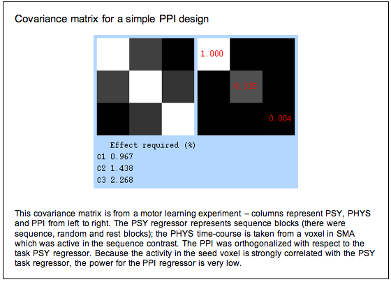
When should you (not) use PPI?
In theory, PPI can be used with any experimental design. However, in practice you are unlikely to see a significant effect in most experimental designs. The reason for this is that, to avoid the confounds described above, you have to include the main effects from which you derived your interaction variable in the GLM. But because the psychological, physiological and interaction variables are now strongly correlated, the design lacks power. You can see this from the covariance matrix below – we would need a signal change of over 2% associated with the interaction term to see a significant effect.
Literature review of PPI
The PPI method was originally reported in 1997 in the following paper:
Friston, Buechel, Fink, Morris, Rolls and Dolan (1997) Psychophysiological and modulatory interactions in neuroimaging Neuroimage 6: 218-229
and has been implemented as a function in SPM since SPM2. A search in the Science Citation Index revealed that of 189 papers citing the original Friston paper, of which 40 were fMRI studies in which PPI had been used, of which 15 were published by people at the FIL and most of the rest had at least one author at the FIL.
If these numbers really reflect the number of studies in which PPI has been used ‘successfully’ (that is, in which there was a significant result), then the number is surprisingly low, given that there is a PPI button in the SPM GUI and given the number of posts about PPI on the SPM mailing list (240). Further, about twice as many papers have been published using PPI with PET as with fMRI. Applying some Bayesian inference based on the proportion of PET to fMRI papers in the literature and the proportion of people likely to be clicking the PPI button to those who got a paper out of it, I have to suspect that this method does not work very successfully with fMRI data. This is probably because of the orthogonality issue described above in non-factorial designs.
Factorial designs
PPI is supposed to work better with factorial designs. The reasons for this are described in Friston (1997), which I quote here:
Psychophysiological interactions generally depend on factorial experimental designs, wherein one can introduce neurophysiological changes in one brain system that are uncorrelated with the stimulus or cognitive context one hopes to see an interaction with. We make this point explicit, suggesting that this is another example of the usefulness of factorial experiments: Although it is possible to test for psychophysiological interactions in almost any experimental design, the use of factorial designs ensures that any psychophysiological interactions will be detected with a fair degree of sensitivity. This is because the activities in the source area, the psychological context, and the interaction between them, will be roughly orthogonal and therefore one can use the first two as confounds with impunity. The converse situation, in which only one stimulus or cognitive factor has been changed, may render the activity in the source area and changes in the factor correlated. If this is the case, there is no guarantee that the interaction will be independent of either and its effect may be difficult to detect in the presence of the "main effects".
This makes sense in some ways, but to me it seems strange – surely the only reason this works is that you are including psychological variables which differ from the contrast of interest, which would after all be the interaction contrast [1, -1/3, -1/3, -1/3] ?
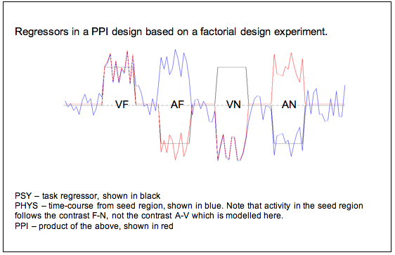
In other words, if we have a factorial design the psychological, physiological and interaction regressors will be relatively orthogonal. Say we are doing an experiment on memory in different sensory modalities, and we have a 2x2 design with factors A vs. V (auditory and visual) and F vs. N (familiar vs. novel stimuli). Then we might define a seed voxel for our PPI which is active in the GLM contrast familiar-novel (perhaps in the medial temporal lobe), and analyse the PPI in the visual condition (perhaps we think visual cortex will show a stronger functional connection with medial temporal lobe in the familiar condition). Then our regressors will be as follows:
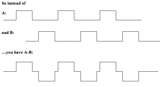
- PSY: task contrast visual-auditory (shown in black below)
- PHYS: time-course from our voxel in medial temporal lobe– this is more active in the familiar condition than the novel condition (shown in blue below)
- PPI: the product of PSY and PHYS.
Because the contrast we used to select the seed region is not the same as the contrast we are interested in in the PPI analysis, our regressors are now looking a lot more orthogonal:
Frequently asked questions
Should I include other task variables in the model?
Generally speaking, yes you should. You should include all the task EVs which were in your GLM model, even those which are not involved in generating your PPI regressor. This will make the model overall a better description of the data. However, in the literature you find papers which do this, and papers which don’t.
I want to show that my ROI interacts with some areas more in condition A than condition B (rather than just showing interaction is greater in condition A than baseline). How do I do that?
Since you can only generate an interaction between two regressors, you will need to make a task regressor (for your PSY EV) which embodies the contrast A-B. In other words, make a 3-column format regressor which has all the task blocks of A and B in it, but the weight (3rd column value) of A is 1 and the weight of B is -1.
Then your regressors will be A-B, your ROI timecourse, and the interaction between ROI timecourse and A-B (as above).
In this case you should not include A and B as well, or your design will be rank deficient.
However, if you are using A-B, you SHOULD also include a regressor for A+B (make it in 3-column format as above with all A's and B's in a single file, but all the A's and B's will have a weight of +1). The reason for doing this is that by including A-B, you can model all the differences between A and B - but not the shared variance. Including A+B mops up this shared variance. In terms of the overall model fit, {A-B and A+B} should give the same overall fit as {A and B} did in your original model. Mathematically, we would say {A+B and A-B} span the same vector space as {A and B}.
This approach should work even if you want to combine more EVs (eg A-(B+C)). Just set the weight of all the ‘minus’ conditions (B and C here) to -1, and the ‘plus’ conditions (A here) to 1 - and be sure to click the zero-centre EV button when you are making your PPI regressor.
Can I include more than one ROI/ PPI in my model?
Not a good idea in general. You are still running a GLM analysis which, as always, rests on the assumption that your regressors are orthogonal (or close to it). Your timecourses are likely not orthogonal, especially if you picked them from the same GLM output. This will screw up your analysis. Instead, run separate analyses for each ROI. You can then compare between them with a higher-level Feat analysis.