Dual regression
Research overview
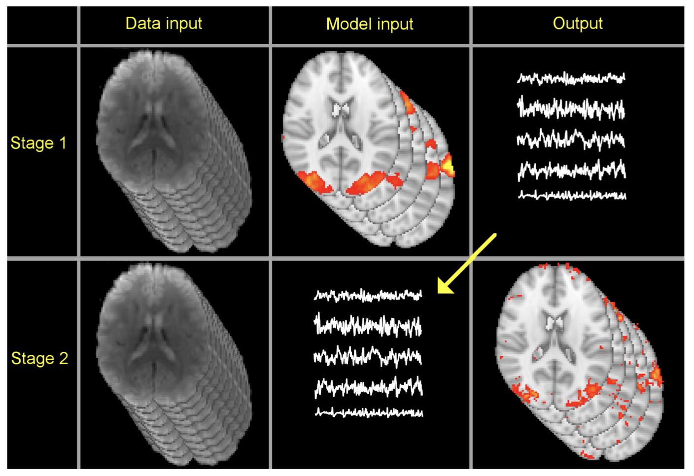
A common way to analyse resting-state FMRI data is to run a group-average ICA, and then, for each subject, estimate a "version" of each of the group-level spatial maps. This can be done with dual regression. This: - Regresses the group-spatial-maps into each subject's 4D dataset to give a set of timecourses (stage 1) - Regresses those timecourses into the same 4D dataset to get a subject-specific set of spatial maps (stage 2)
The spatial maps can be then used for group-level analyses, for example comparinig maps across groups of subjects to look for group differences using randomise permutation testing (this can be done with the dual_regression command as "stage 3").
Referencing
If you use dual regression in your research, please make sure that you reference at least one of the articles listed below. For your convenience, we provide example text, which you are welcome to use in your methods description.
"The set of spatial maps from the group-average analysis was used to generate subject-specific versions of the spatial maps, and associated timeseries, using dual regression [Beckmann2009,Filippini2009, Nickerson2017]. First, for each subject, the group-average set of spatial maps is regressed (as spatial regressors in a multiple regression) into the subject's 4D space-time dataset. This results in a set of subject-specific timeseries, one per group-level spatial map. Next, those timeseries are regressed (as temporal regressors, again in a multiple regression) into the same 4D dataset, resulting in a set of subject-specific spatial maps, one per group-level spatial map. We then tested for [group differences, etc.] using FSL's randomise permutation-testing tool."
- [Beckmann2009] C.F. Beckmann, C.E. Mackay, N. Filippini, and S.M. Smith. Group comparison of resting-state FMRI data using multi-subject ICA and dual regression. OHBM, 2009 Pdf
- [Filippini2009] N. Filippini, B.J. MacIntosh, M.G. Hough, G.M. Goodwin, G.B. Frisoni, S.M. Smith, P.M. Matthews, C.F. Beckmann, C.E. Mackay. Distinct patterns of brain activity in young carriers of the APOE-epsilon4 allele. Proc. Natl. Acad. Sci. U. S. A., 106 (2009), pp. 7209-7214
- [Nickerson2017] L. Nickerson, S.M. Smith, D. Öngür, C.F. Beckmann. Using Dual Regression to Investigate Network Shape and Amplitude in Functional Connectivity Analyses. Front Neurosci. 2017; 11: 115. doi: 10.3389/fnins.2017.00115
User guide
Running Dual Regression
- Run MELODIC on your group data in Concat-ICA mode ("Multi-session temporal concatenation"). Find the file containing the ICA spatial maps output by the group-ICA; this will be called something like
melodic_IC.nii.gzand will be inside asomething.icaMELODIC output directory. - Use
Glm(or any other method) to create your multi-subject design matrix and contrast files (design.mat/design.con). -
Run dual_regression. Simply type
dual_regressionto get the usage:Usage: dual_regression <group_IC_maps> <des_norm> <design.mat> <design.con> <n_perm> [--thr] <output_directory> <input1> <input2> <input3> ......... e.g. dual_regression groupICA.gica/groupmelodic.ica/melodic_IC 1 design.mat design.con 500 0 grot `cat groupICA.gica/.filelist` <group_IC_maps_4D> 4D image containing spatial IC maps (melodic_IC) from the whole-group ICA analysis <des_norm> 0 or 1 (1 is recommended). Whether to variance-normalise the timecourses used as the stage-2 regressors <design.mat> Design matrix for final cross-subject modelling with randomise <design.con> Design contrasts for final cross-subject modelling with randomise <n_perm> Number of permutations for randomise; set to 1 for just raw tstat output, set to 0 to not run randomise at all. [--thr] Perform thresholded dual regression to obtain unbiased timeseries for connectomics analyses (e.g., with FSLnets) <output_directory> This directory will be created to hold all output and logfilesg <input1> <input2> ... List all subjects' preprocessed, standard-space 4D datasets <design.mat> <design.con> can be replaced with just -1 for group-mean (one-group t-test) modelling. If you need to add other randomise options then edit the line after "EDIT HERE" in the dual_regression script- The 4D group spatial IC maps file will be something like
somewhere.ica/melodic_IC - The
des_normoption determines whether to variance-normalise the timecourses created by stage 1 of the dual regression; it is these that are used as the regressors in stage 2. If you don't normalise them, then you will only test for RSN "shape" in your cross-subject testing. If you do normalise them, you are testing for RSN "shape" and "amplitude". - One easy way to get the list of inputs (all subjects' standard-space 4D timeseries files) at the end of the command is to use the following (instead of listing the files explicitly, by hand), to get the list of files that was fed into your group-ICA:
cat somewhere.gica/.filelist
- The 4D group spatial IC maps file will be something like
Explanation of outputs
dr_stage1_subject[#SUB].txt- the timeseries outputs of stage 1 of the dual-regression. One text file per subject, each containing columns of timeseries - one timeseries per group-ICA component. These timeseries can be fed into further network modelling, e.g., taking the N timeseries and generating an NxN correlation matrix.dr_stage2_subject[#SUB].nii.gz- the spatial maps outputs of stage 2 of the dual-regression. One 4D image file per subject, and within each, one timepoint (3D image) per original group-ICA component. These are the GLM "parameter estimate" (PE) images, i.e., are not normalised by the residual within-subject noise. By default we recommend that it is these that are fed into stage 3 (the final cross-subject modelling).dr_stage2_subject[#SUB]_Z.nii.gz- the Z-stat version of the above, which could be fed into the cross-subject modelling, but in general does not seem to work as well as using the PEs.dr_stage2_ic[#ICA].nii.gz- the same as the PE images described above, but reorganised into being one 4D image file per group-ICA component, and, within each, having one timepoint (3D image) per subject. This reorganisation is to allow stage 3, the cross-subject modelling for each group-ICA component - so it is these files that would normally be fed into randomise.dr_stage3_ic[#ICA]_tstat[#CON].nii.gz- the output of "stage 3", i.e. files created by running randomise, doing cross-subject statistics separately for each group-ICA component. You'll get one set of statistical output files per group-ICA component, and, within that set of statistical output files, one t-stat (etc.) per contrast in the cross-subject contrast file (design.con). The corresponding corrected (1-p) p-value images are called*corrp*.
Multiple-comparison correction across all RSNs
The need for correction, and correction via Bonferroni
Warning: The corrected p-values output by the final randomise (corrp) are fully corrected for multiple comparisons across voxels, but only for each RSN in its own right, and only doing one-tailed testing (for t-contrasts specified in design.con).
This means that if you test (with randomise) all components found by the initial group-ICA, and you do not have a prior reason for only considering one of them, you should correct your corrected p-values by a further factor. For example, let's say that your group-ICA found 30 components, and you decided to ignore 18 of them as being artefact. You therefore only considered 12 RSNs as being of potential interest, and looked at the outputs of randomise for these 12, with your model being a two-group test (controls and patients). However, you didn't know whether you were looking for increases or decreases in RSN connectivity, and so you ran the two-group contrast both ways for each RSN. In this case, instead of your corrected p-values needing to be <0.05 for full significance, they really need to be < 0.05 / (12 * 2) = 0.002 !
FAQ
What does it mean if I find a dual-regression result outside a given RSN?
For example, if you have two groups of subjects (patients and controls), did a group-ICA on the basis of all subjects from both groups, and then run dual-regression. You then did a two-group t-test using the spatial maps output by dual-regression, and found a significant difference for one of the RSNs. However, what does it mean if the voxels showing a significant difference are not "within" the (group-average) ICA map for that RSN? This is not necessarily indicative of a problem at all (as long as it's in grey matter!). It just means that the "connectivity" of this area with the main regions of this RSN is different in the two groups, despite on average (across both groups) not being strongly connected. For example, this area might have a weak positive correlation with the main areas of this RSN in the control group, and a weak negative correlation in the patient group.