FAST

FAST (FMRIB's Automated Segmentation Tool) segments a 3D image of the brain into different tissue types (Grey Matter, White Matter, CSF, etc.), whilst also correcting for spatial intensity variations (also known as bias field or RF inhomogeneities). The underlying method is based on a hidden Markov random field model and an associated Expectation-Maximization algorithm. The whole process is fully automated and can also produce a bias field-corrected input image and a probabilistic and/or partial volume tissue segmentation. It is robust and reliable, compared to most finite mixture model-based methods, which are sensitive to noise.

If you use FAST in your research, please cite the following article:

Zhang, Y. and Brady, M. and Smith, S. Segmentation of brain MR images through a hidden Markov random field model and the expectation-maximization algorithm. IEEE Trans Med Imag, 20(1):45-57, 2001

The different FAST programs are Fast (Fast_gui on macOS) for the GUI, and fast for the command-line program

Before running FAST an image of a head should first be brain-extracted, using BET. The resulting brain-only image can then be fed into FAST.

Fast GUI

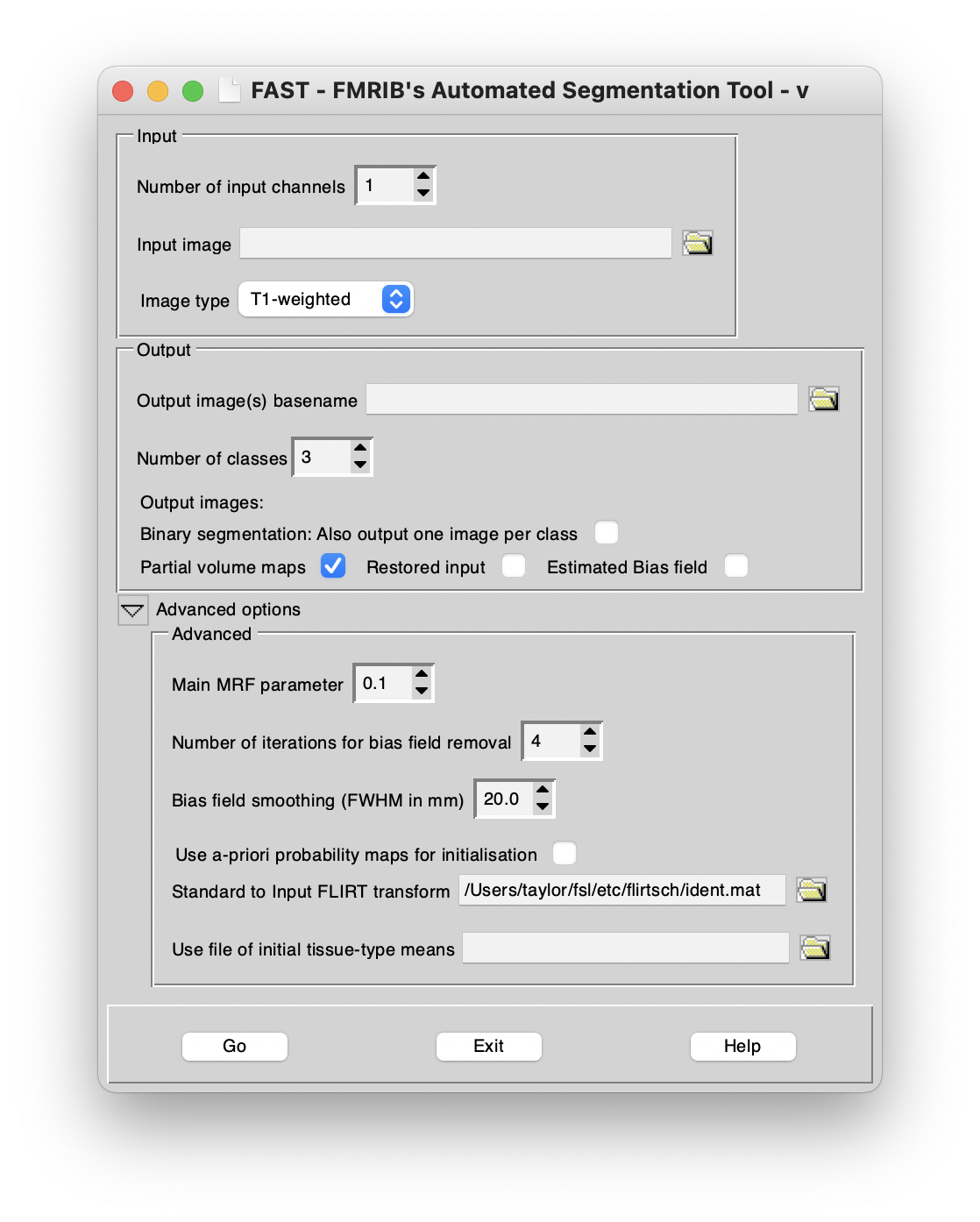
Main options

If there is only one input image (i.e., you are not carrying out multi-channel segmentation) then leave the Number of input channels at 1. Otherwise, set appropriately.

Now select the Input image(s).

Now set the Image type. This aids the segmentation in identifying which classes are which tissue type. Note that this option is not used for multi-channel segmentation.

Now select the Output image(s) basename. Output images will have filenames derived from this basename. For example, the main ouput, the Binary segmentation: All classes in one image will have filename <basename>_seg. If multi-channel segmentation is carried out, some of the optional outputs will have basenames derived instead from the input names (but into the directory of the outputbasename). For example, the main segmentation output will be as described above, but the restored images (one for each input image) will be named according to the input images.

Now choose the Number of classes to be segmented. Normally you will want 3 (Grey Matter, White Matter and CSF). However, if there is very poor grey/white contrast you may want to reduce this to 2; alternatively, if there are strong lesions showing up as a fourth class, you may want to increase this. Also, if you are segmenting T2-weighted images, you may need to select 4 classes so that dark non-brain matter is processed correctly (this is not a problem with T1-weighted as CSF and dark non-brain matter look similar).

The various output options are:

• Partial volume maps: A (non-binary) partial volume image for each class, where each voxel contains a value in the range 0-1 that represents the proportion of that class's tissue present in that voxel. This is the default output.
• Binary segmentation:single image: This is the "hard" (binary) segmentation, where each voxel is classified into only one class. A single image contains all the necessary information, with the first class taking intensity value 1 in the image, etc.
• Binary segmentation: One image per class: This is also a hard segmentation output; the difference is that there is one output image per class, and values are only either 0 or 1.
• Restored input: This is the estimated restored input image after correction for bias field.
• Bias field: This is the estimated bias field.

Advanced options

Bias field iterations determines the number of passes made during the initial bias field estimation stage. A greater number of iterations can help esitmate particularly strong bias fields.

Bias field smoothing controls the amount of smoothness expected in the estimated bias field. The value entered is the Full-Width Half-Maximum (FWHM) in mm. A larger value here will impose more smoothness on the estimated bias field.

Use a-priori probability maps tells FAST to start by registering the input image to standard space and then use standard tissue-type probability maps (from the MNI152 dataset) instead of the initial K-means segmentation, in order to estimate the initial parameters of the classes. This can help in cases where there is very bad bias field. By default the a-priori probability maps are only used to initialise the segmentation; however, you can also optionally tell FAST to use these priors in the final segmentation - this can help, for example, with the segmentation of deep grey structures.

Use file of initial tissue-type means tells FAST to use a text file with mean intensity values (separated by newlines) for the starting mean values of the different classes to be segmented. This is then used instead of the automated K-means starting parameter estimation.

Fast command-line program

Type fast to get usage. The is used for both single-channel and multi-channel segmentation.

Main inputs/options

Usage:
fast [options] file(s)

Optional arguments (You may optionally specify one or more of):
    -n,--class  number of tissue-type classes; default=3
    -t,--type   type of image 1=T1, 2=T2, 3=PD; default=T1
    -b      output estimated bias field
    -B      output bias-corrected image
    -S,--channels   number of input images (channels); default 1
    -o,--out    output basename

Advanced options:

    -a <standard2input.mat> initialise using priors; you must supply a FLIRT transform
    -P,--Prior  use priors throughout; you must also set the -a option
    -R,--mixel  spatial smoothness for mixeltype; default=0.3
    -H,--Hyper  segmentation spatial smoothness; default=0.1
    -s,--manualseg <filename> Filename containing intensities

Tissue volume quantification

Estimating the tissue volume for a given class can be done using FAST and we recommend using the partial volume estimates for the most accurate quantification. The actual volume of tissue can be calculated easily from the corresponding partial volume map by summing up all the values. This can be done using fslstats and then multiplying the mean value by the volume (in voxels).

For example, for an image called structural_bet that fast was run on, the tissue volume of tissue class 1 can be found by running the following:

vol=`$FSLDIR/bin/fslstats structural_bet_pve_1 -V | awk '{print $1}'`
mean=`$FSLDIR/bin/fslstats structural_bet_pve_1 -M`
tissuevol=`echo "$mean * $vol" | bc -l`
echo $tissuevol

This prints the total tissue volume in voxels (which is also stored in the variable tissuevol). Note that to get the volume in mm³ just replace the {print $1} with {print $2} in the first line above. Alternatively, this can be done in the single line:

fslstats structural_bet_pve_1 -M -V | awk '{ print $1 * $3 }'