FIRST

FIRST is a model-based segmentation/registration for automatic segmentation of a number of subcortical structures.

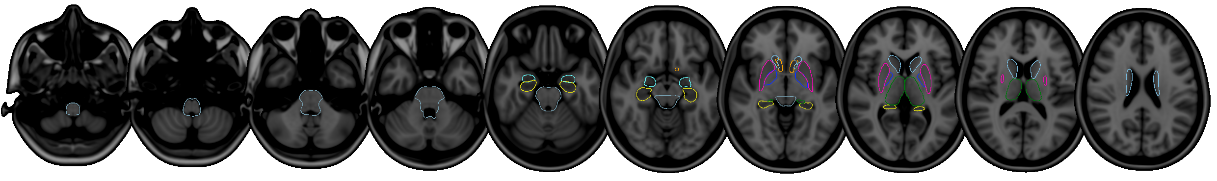
The supported structures are listed below. To segment these structures, FIRST needs a good quality T1-weighted image:

• Putamen (Puta)
• Caudate nucleus (Caud)
• Nucleus accumbens (Accu)
• Globus pallidus (Pall)
• Hippocampus (Hipp)
• Amygdala (Amyg)
• Thalamus (Thal)
• Brainstem (BrStem)

The outputs produced by FIRST can be fed into a range of different analyses, including: - Vertex analysis, which allows one to explore localised differences in structural shape. - Volumetric analysis, which can be used to compare the volume of structures across groups.

The shape/appearance models used in FIRST are constructed from manually segmented images provided by the Center for Morphometric Analysis (CMA), MGH, Boston. The manual labels are parameterized as surface meshes and modelled as a point distribution model. Deformable surfaces are used to automatically parameterize the volumetric labels in terms of meshes; the deformable surfaces are constrained to preserve vertex correspondence across the training data. Furthermore, normalized intensities along the surface normals are sampled and modelled. The shape and appearance model is based on multivariate Gaussian assumptions. Shape is then expressed as a mean with modes of variation (principal components). Based on our learned models, FIRST searches through linear combinations of shape modes of variation for the most probable shape instance given the observed intensities in a T1-weighted image.

For more information on FIRST, see the NeuroImage paper - the following reference is the main journal paper describing FIRST:

Patenaude, B., Smith, S.M., Kennedy, D., and Jenkinson M. A Bayesian Model of Shape and Appearance for Subcortical Brain NeuroImage, 56(3):907-922, 2011.

There is also a thesis relating to FIRST that contains some more technical details:

Brian Patenaude. Bayesian Statistical Models of Shape and Appearance for Subcortical Brain Segmentation. D.Phil. Thesis. University of Oxford. 2007.

We are very grateful for the training data for FIRST, particularly to David Kennedy at the CMA, and also to: Christian Haselgrove, Centre for Morphometric Analysis, Harvard; Bruce Fischl, Martinos Center for Biomedical Imaging, MGH; Janis Breeze and Jean Frazier, Child and Adolescent Neuropsychiatric Research Program, Cambridge Health Alliance; Larry Seidman and Jill Goldstein, Department of Psychiatry of Harvard Medical School; Barry Kosofsky, Weill Cornell Medical Center.

Supported structures

The structures that FIRST can segment are listed below. The Abbrevbiated name column gives the name that you should pass to the FIRST command-line tools when you want to segment a specific structure. The Integer label column gives the integer label that FIRST assigns to each structure in its output files (e.g. output_*_firstseg.nii.gz). The Modes column gives the recommended number of modes of variation to use for each structure when fitting the subcortical model (note that this is normally taken care of automatically for you).

Structure	Abbreviated name	Integer label	Modes
Left Thalamus	L_Thal	10	40
Left Caudate	L_Caud	11	30
Left Putamen	L_Puta	12	40
Left Pallidum	L_Pall	13	40
Brain Stem	BrStem	16	40
Left Hippocampus	L_Hipp	17	30
Left Amygdala	L_Amyg	18	50
Left Accumbens	L_Accu	26	50
Right Thalamus	R_Thal	49	40
Right Caudate	R_Caud	50	30
Right Putamen	R_Puta	51	40
Right Pallidum	R_Pall	52	40
Right Hippocampus	R_Hipp	53	30
Right Amygdala	R_Amyg	54	50
Right Accumbens	R_Accu	58	50

Segmentation with run_first_all

The simplest way to perform segmentation using FIRST is to use the run_first_all script. This script segments all the subcortical structures, producing mesh and volumetric outputs (applying boundary correction to produce the volumetric segmentations). It uses default settings for each structure which have been optimised empirically.

This script will run lower-level utilities (including first_flirt, run_first and first) on all the structures, with the settings (number of modes and boundary correction) tuned to be optimal for each structure. Both mesh (vtk) and volumetric (nii.gz) outputs are generated. Corrected and uncorrected volumetric representations of the native mesh are generated. The final stage of the script ensures that there is no overlap between structures in the 3D image, which can occur even when there is no overlap of the meshes, as can be seen in the individual, uncorrected segmentation images in the 4D image file.

Example usage:

run_first_all -i t1_image -o output_name

• The argument -i specifies the original T1-weighted structural image (only T1-weighted images can be used).

• The argument -o specifies the filename for the output image basename. run_first_all will include the type of boundary correction into the final file name. For example, the command above would produce output_name_all_fast_firstseg.nii.gz and output_name_all_fast_origsegs.nii.gz.

The script is written such that if you have FSL setup to use local cluster computing it will automatically parallelise the fitting of each structure. Either way, it will create a log directory that contains the error outputs of each command, and you should check these. To do that simply run:

cat *.logs/*.e*

and if there are no errors then you will see no output, otherwise you will see what errors have occured.

The run_first_all scripts accepts the following additional options:

• -m specifies the boundary correction method. The default is auto, which chooses different options for different structures using the settings that were found to be empirically optimal for each structure. Other options are: fast (using FAST-based, mixture-model, tissue-type classification); thresh (thresholds a simple single-Gaussian intensity model); or none.

• -s allows a restricted set of structures (one or more) to be selected. For more than one structure the list must be comma separated with no spaces. The list of possible structures is: L_Accu L_Amyg L_Caud L_Hipp L_Pall L_Puta L_Thal R_Accu R_Amyg R_Caud R_Hipp R_Pall R_Puta R_Thal BrStem.

• -b specifies that the input image is brain extracted - important when calculating the registration.

• -a specifies a pre-calculated registration matrix (from running first_flirt) to be used instead of calculating the registration again.

Output files

The run_first_all script produces the following output files:

• output_name_all_fast_firstseg.nii.gz: This is a single image showing the segmented output for all structures. The image is produced by filling the estimated surface meshes and then running a step to ensure that there is no overlap between structures. The output uses the labels listed above (and a standard colour table is built into FSleyes). If another boundary correction method is specified, the name fast in this filename will change to reflect the boundary correction that is used. Note that if only one structure is specified then this file will be called output_name-struct_corr.nii.gz instead (e.g. sub001-L_Caud_corr.nii.gz).

• output_name_all_fast_origsegs.nii.gz: This is a 4D image containing the individual structure segmentations, converted directly from the native mesh representation and without any boundary correction. For each structure there is an individual 3D image where the interior is labeled according to the CMA standard labels while the boundary uses these label values plus 100. Note that if only one structure is specified then this file will be called output_name-struct_first.nii.gz instead (e.g. sub001-L_Caud_first.nii.gz).

• output_name_first.vtk : This is the mesh representation of the final segmentation. It can be loaded into FSLeyes and overlaid on your T1 image.

• output_name_first.bvars: Do not delete this file. It contains the mode parameters and the model used. This file, along with the appropriate model files, can be used to reconstruct the other outputs. The mode parameters are what FIRST optimizes. This output can be used be used later as to perform vertex analysis or as a shape prior to segment other shapes.

General advice and workflow

Below is a recommendation for running FIRST in a systematic way. While it is only a recommendation, you may find that organizing your data in a different way than suggested below leads to complications further down the road, especially when moving files.

• Create a main directory in which the FIRST analysis will be carried out. The first step in analysis will be to copy all of the structural images to be segmented into this directory. All FIRST commands should be run in this directory. Subdirectories may be created to contain certain outputs (more later) but all input images should be placed in this main directory. The pathnames for files used as input options for all of the steps of FIRST should start in this directory and may include subdirectories as needed. The reason for this is that the pathnames of the structural input images are written into the bvars output files. When these bvars files are used (i.e. for vertex analysis), the original image must be able to be located. Inputting full pathnames is possible, but if you move the directory containing the structural images, the pathnames within the bvars files will have to be changed. Therefore, we recommend keeping all FIRST inputs and outputs in one main directory and keeping all pathnames relative to this directory. This way, if the entire directory is moved then the relative position of all input and output files will remain the same.

For example, imagine you have a directory called scratch, and you create a sub-directory called subcort. Start by copying all of your images into the subcort directory. Once this is done, all subsequent steps should be carried out from within the directory subcort.

• Use a standardized naming system for all of your structural images and subsequent output files. For example, we will consider an experiment where there are 10 controls and 10 diseased subjects. In this case we name the structural images con01.nii.gz, con02.nii.gz, ..., dis01.nii.gz, dis02.nii.gz, ... and keep the base name part (e.g. con01) the same for all outputs of FIRST.

• To run run_first_all on a group of subjects a simple for loop may be used from the command line, for example:

  for i in 01 02 03 04 05 06 07 08 09 10 ; do
      run_first_all -i con${i} -o con${i} ;
  done
  

  A similar loop can then be run for the diseased subjects (dis01, ..., dis10). These commands could be put into one big for loop, but it is usually simpler to separate them, especially if you have a different number of subjects in each group.

• You then need to verify that the registrations and subsequent segmentations were successful. To start with, check that there are no errors in the log files by doing:

  cat *.logs/*.e*
  

which will show no output if there are no errors.

• Once you've verified that there are no errors, then you can most easily check the quality of the registrations using the slicesdir tool:

  slicesdir -p ${FSLDIR}/data/standard/MNI152_T1_1mm.nii.gz *_to_std_sub.nii.gz
  

This command creates a directory called slicesdir which will contain a webpage output of the summary results for each subject's registration. Note that if the registration stage failed then the model fitting will not work, even though run_first_all will continue to run and generate output. Therefore it is critical to check the registration results.

On the webpage, each subject's registered image (*_to_std_sub.nii.gz) will be displayed in sagittal, coronal, and axial views, with a red outline showing the edges from the MNI152_T1_1mm standard brain. Open this webpage in any web browser.

When assessing the registrations, pay particular attention to the sub-cortical structures. It does not matter if the cortex does not always align well, particularly where there are large ventricles, as it is the alignment of the sub-cortical structures which is important for the segmentation.

• To check the segmentations, firstly, fix any registration errors (see below for first_flirt and various options available) and re-run the segmentation using the new registration. After that the segmentation output can be inspected. This can be done using first_roi_slicesdir which generates a similar webpage to slicesdir, but this time showing the segmentations. first_roi_slicesdir is a script to generate summary images, in a webpage format, for the segmentation outputs. It is very useful for checking the quality of segmentations, especially when there are many subjects. It runs the script slicesdir on a region of interest (ROI) defined by a set of label images (e.g. output of FIRST). A set of temporary ROI images are created and then slicesdir is then run on those. You can use first_roi_slicesdir like so:

  first_roi_slicesdir <list of t1_images> <list of label_images>
  

  For example:

  first_roi_slicesdir *_t1.nii.gz *_all_fast_firstseg.nii.gz
  

If there are any problems, you can try different segmentation options (e.g. number of modes, boundary correction method, etc.) using the individual tools described in the Advanced Usage section.

Comparing shape differences using vertex analysis

This section describes how to calculate vertex-wise statistics to investigate localised shape differences. In brief, a vertex analysis workflow proceeds as follows:

1. Use run_first_all to produce sub-cortical segmentmentations for all of your subjects
2. Use concat_bvars to combine all of the bvars files for a given structure from each subject into a single file.
3. Create a design matrix, for example, usign the Glm GUI.
4. Use first_utils to convert the concatenated bvars file into a nii.gz file, suitable for passing to randomise.
5. Use randomise to perform the statistical analysis.

Vertex analysis is performed using first_utils in a mode of operation that aims to assess group differences on a per-vertex basis. It uses randomise to do the statistical analysis. The simplest, and very common, design matrix is a single EV (regressor) specifying group membership (-1 for one group, +1 for the other group) together with a single F-contrast (also requiring a single t-contrast) which then tests for group differences in a two-sided (unsigned) test. Any of the many available multiple comparison correction techniques available in randomise can be used (some method of correction should be used if presenting results in a publication).

The output of the first_utils command is a 4D image that are can be processed via randomise. The corrp image outputs from randomise display 1-p values (so that over 0.95 is "significant" at the 0.05 level). Results are only displayed on the structure's surface.

Internally the vertex locations from each subject (at a corresponding anatomical point) are projected onto the surface normal of the average shape (of this particular cohort). The projections are scalar values, allowing them to be processed by univariate statistical methods (e.g. randomise). It is these projection values that are stored in the 4D file (one image per subject) and they represent the signed, perpendicular distance from the average surface, where a positive value is outside the surface and a negative value is inside. A mask file (covering the vertices on the surface of the average shape) is also produced.

concat_bvars

concat_bvars is used to concatenate the .bvars files across subjects. All subjects should be created using the same model and concat_bvars will keep track of the number of subjects that the final, concatenated file contains. Usage is as follows:

concat_bvars output_name.bvars [list of ".bvars" files]

For example:

concat_bvars L_Hipp_all.bvars con*_L_Hipp_first.bvars dis*_L_Hipp_first.bvars

first_utils

Usage of the first_utils command is as follows:

first_utils --vertexAnalysis                    \
            --usebvars                          \
            -i concatenated_bvars               \
            -o output_basename                  \
            -d design.mat                       \
            [--useReconNative --useRigidAlign ] \
            [--useReconMNI]                     \
            [--saveAverageMesh]                 \
            [--usePCAfilter -n number_of_modes]

The options used for vertex analysis as follows:

• --vertexAnalysis: Set mode of operation such that vertex-wise stats are calculated.

• --usebvars : Set mode of operation such that it uses the combined mode parameters across the group (this is compulsory for vertex analysis).

• -i concatenated_bvars: concatenated bvars file containing mode parameters from all subjects (created by concat_bvars).

• -o output_basename: Base name of output meshes.

• -d design.mat: FSL design matrix (e.g. as created by the Glm GUI).

• --useReconNative: Reconstructs the meshes in the native space of the image. For vertex-wise stats need to also use --useRigidAlign.

• --useReconMNI: Reconstructs the meshes in MNI space (native space of the model). This does not require the flirt matrices.

• --useRigidAlign: Uses a 6 Degrees Of Freedom transformation to remove pose from the meshes (see --useScale if you wish to remove size as well). All meshes are aligned to the mean shape from the shape Model. Can be used with either --useReconNative or --useReconMNI.

• --useScale: Used in conjunction with --useRigidAlign, it will remove global scalings when aligning meshes.

• --usePCAfilter: Used in conjunction with -n number_of_modes. When used the number of modes used to reconstruct the mesh will be truncated at the integer number_of_modes.

• --saveAverageMesh : Save the group average mesh as a VTK file - this is useful for visualising results.

The outputs from first_utils are images suitable for statistical testing in randomise. It is still necessary to specify a design matrix (but not contrasts) for first_utils, whereas both a design matrix and contrasts are necessary for the randomise step.

randomise

The randomise command is used to calculate the statistics from the 4D image produced by first_utils. This requires design matrix, t-contrast and f-contrast files to be specified. These can be created by the Glm GUI.

Example usage is as follows:

randomise -i con1_dis2_L_Hipp.nii.gz      \
          -m con1_dis2_L_Hipp_mask.nii.gz \
          -o con1_dis2_L_Hipp_rand        \
          -d con1_dis2.mat                \
          -t con1_dis2.con                \
          -f con1_dis2.fts                \
          --fonly -D -F 3

Here the -d, -t, and -f flags specify the files containing the design matrix, t-contrast(s) and f-contrast(s). The -D option demeans the data (and design matrix - you can ignore the warning about the design having a non-zero mean, as this will be removed internally and give correct outputs). The -F 3 option does cluster-based multiple-comparison-correction (with an arbitrary threshold of 3, which is only an example here) but could be substituted with any other valid multiple-comparison-correction option such as --T2, -x, -S. See the randomise documentation for more information on available options.

The --fonly option is included so that only the F-statistic is calculated and used by randomise for inference. This is then equally sensitive to changes in either direction (e.g., growth or atrophy). To determine which direction the change is in there are two possible approaches:

1. omit this option and look at the t-contrast results (carefully taking into account the signs used in both the design matrix EVs and the contrast) or;
2. more simply, just look at the signs of the individual data points in the 4D input file.

The second option is generally easier and is quite simply done with FSLeyes, by loading the corrected p-value output from randomise (the f-statistic result, having kept the --fonly option) then adding the 4D input file and using the "timeseries" view in FSLeyes to see the values from the 4D input file at boundary locations where there was a statistically significant change.

General advice and workflow

This section covers some general recommendations for running vertex analysis. The following is not prescriptive but may be helpful, especially to new users or those less familiar with unix-style commands and environments.

Getting started

To begin with you need to generate segmentations of all the structure of interest in all subjects (see the segmentation section). Note that it is the bvars files, which correspond directly to the surface representations, which will be needed - the volumetric representation from FIRST (e.g. run_first_all) is not used. Hence it does not matter what boundary correction was used or whether one or more structures were segmented.

One the segmentations are done, concatenate all of the bvars files for the structure you are going to run vertex-wise stats on. For example if you are looking for differences in the left hippocampus, and assuming your output bvars files are named con*_L_Hipp_first.bvars and dis*_L_Hipp_first.bvars, do:

concat_bvars con_to_dis_L_Hipp.bvars con*_L_Hipp_first.bvars dis*_L_Hipp_first.bvars

This command will create a bvars file called con_to_dis_L_Hipp.bvars that contains the bvars (mode paramters) of the segmentation of the left hippocampus from each subject in the order con01-con10, followed by dis01-dis10.

Create a design matrix

This is easiest done by using the Higher-level mode of the Glm GUI. However, the design matrices are treated slightly differently by FIRST compared with FEAT. The main difference is that FIRST does not model separate group variances and so ignores the Group column in the Glm GUI. Another difference is that only F-tests are needed if you just want to look for any change in vertex position. Therefore it is only necessary to set up an F-contrast, although this needs T-contrasts to be set up (since that is how F-contrasts are specified). Individual T-contrasts can be used to look for signed differences (separating local "expansion" from "contraction" of the structure). For more details about this see the FEAT documention.

For this example, imagine you are simply interested in finding a difference in shape between the two groups "con" and "dis". Your design matrix would simply be an EV with 10 negative ones followed by 10 positive ones. That is:

-1
-1
-1
-1
-1
-1
-1
-1
-1
-1
1
1
1
1
1
1
1
1
1
1

Create this design (using the Glm GUI) and specify both a single T-contrast and single F-contrast, and then save them in files named con1_dis2 (choose the name con1_dis2 in the Save dialog of the Glm GUI - it will produce con1_dis2.mat, con1_dis2.con and con1_dis2.fts). Note that because the concatenated bvars files was created in the order con, then dis, in your design matrix group 1 is the con group and group 2 is the dis group.

You are now ready to run vertex_analysis. Note that for this example, the --useReconNative option will be used. This carries out vertex analysis in native space, along with the --useRigidAlign option. The --useReconMNI option may also be used to carry out vertex analysis, it will do it in the MNI standard space instead, which normalises for brain size. It is difficult to say which will be more sensitive to changes in shape, and so it may be interesting to try both the --useReconNative and the --useReconMNI options. Also note that the --useScale option will not be used. Without the --useScale option, changes in both local shape and size can be found in shape analysis. This type of finding can be interpreted, for example, as local atrophy. With the --useScale option, overall changes in size are lost.

Create a new directory (e.g. called shape_analysis) within the current main directory. This will be where the results of shape analysis are saved. For example:

mkdir shape_analysis

Running vertex analysis

Run first_utils giving it the combined bvars file and the design matrix. For example:

first_utils --vertexAnalysis                   \
            --usebvars                         \
            -i con_to_dis_L_Hipp.bvars         \
            -d con1_dis2.mat                   \
            -o shape_analysis/con1_dis2_L_Hipp \
            --useReconNative                   \
            --useRigidAlign                    \
            --saveAverageMesh                  \
            -v >& shape_analysis/con1_dis2_L_Hipp_output.txt

Run randomise using the output 4D image (containing projections of the vertex displacements per subject) and the mask image, together with the design matrix and contrast files. For example:

randomise -i con1_dis2_L_Hipp.nii.gz      \
          -m con1_dis2_L_Hipp_mask.nii.gz \
          -o con1_dis2_L_Hipp_rand        \
          -d con1_dis2.mat                \
          -t con1_dis2.con                \
          -f con1_dis2.fts                \
          --fonly -D -F 3

Note that the option -F 3 is only one of several multiple-comparison-correction options available, and this is just an example, not a standard recommendation.

Output of vertex analysis

In the same way as in FSL-VBM and TBSS, randomise is used to generate the statistics. The output of most interest is the probability that is corrected for multiple comparisons. This will contain corrp in the filename. The values within this file contain 1-p values, such that p=0.05 corresponds to a value of 0.95, and so displaying all values over 0.95 with FSLeyes will show the significant areas. For more information about how to view these results refer to the documentation for randomise, FSL-VBM or TBSS.

Other common design matrices

Correlation

For correlation only (no group difference) you can create a design matrix with one column (EV) where each row contains the value of the correlating measure for each subject in the same order as the subject's bvars (in the concatenated bvars file). For example, to correlate age with shape, the design matrix would contain one EV, which would be a single column where each row has the age of each subject in the same order as the concatenated bvars file. If you have not removed the mean from the age values (i.e. demeaned them), then randomise will do it for you, although it will print a warning to this effect (which you can ignore).

Interpretting the results of a correlation: the values in the p-value images will give the probability of a zero correlation (the null hypothesis) at each vertex. You can also do correlation with a covariate (see below). This gives you the same type of output statistics, but accounting for the covariates/confounds.

Covariate

To add a covariate to a group difference study, simple add a second column to the group difference design matrix. This second column should contain the demeaned scores (for each subject in the same order as the concatenated bavrs file) of the measure you wish to use as a covariate; for example, age. If you want to model different correlations in the different groups then you need a separate (demeaned) EV of scores per group. This is the same as any standard GLM analysis, as are the contrasts, except that the final contrast of interest should always be made into an F-contrast (if it is not naturally one already) in order to do a two-sided test. See other documentation on the GLM and modelling for more information.

Viewing results

Results from randomise can be viewed in the standard orthographic or lightbox views in FSLeyes. To distinguish the direction of the changes see the description in the section on randomise above.

Viewing results in 2D

A useful option when displaying statistical results is to view the statistic image (e.g. the f-statistic, t-statistic image, etc), and to highlight significant regions with the corrected P-value image. This can be accomplished in FSLeyes like so:

1. Start up FSLeyes, and add the following as overlays, ensuring that they are ordered in this way in the overlay list:
2. the corrected P value image, e.g. con1_dis2_L_Hipp_rand_clustere_corrp_fstat1.nii.gz
3. the statistic image that you want to visualise, e.g. con1_dis2_L_Hipp_rand_fstat1.nii.gz to display the F-statistics from the randomise call above.
4. The MNI152 1mm standard template
5. Open the overlay display dialog (the gear button at top-left).
6. Select the P-value image in the overlay list, and in the overlay display dialog change these settings:
7. Overlay data type to 3D/4D mask image
8. Show outline only selected
9. Select the statistic image in the overlay list, and in the overlay display dialog adjust the display settings as desired - for example, you can set up a red/blue positive/negative colour display suitable for many statistic values with the following settings:
10. -ve colour map selected
11. First colour map set to Red-Yellow
12. Second colour map set to Blue-Light blue
13. Modulate alpha by intensity selected - this causes regions with a low value to be made transparent
14. Display range and Modulate range adjusted as desired

Viewing results in 3D

You can also visualise results in the FSLeyes 3D view. The best results are achieved by using the --saveAverageMesh option when calling first_utils - this will save a group-average surface representation of the structure being analysed, with a file name that ends with _average.vtk (e.g. shape_analysis/con1_dis2_L_Hipp_average.vtk in the first_utils call above).

1. Start up FSLeyes, open a 3D view (Views -> 3D View), and add the following as overlays:
2. The MNI152 1mm standard template
3. The group average surface, e.g. shape_analysis/con1_dis2_L_Hipp_average.vtk.
4. the statistic image that you want to visualise, e.g. con1_dis2_L_Hipp_rand_fstat1.nii.gz.
5. Select the MNI152 template in the overlay list, open the overlay display dialog (the gear button at top-left), and add some clipping planes to hide portions of the MNI152 as needed. For example, to hide the entire left hemisphere, set the Number of clipping planes to 1, and then set the Clip rotation to 90, and the Clip Z angle to -90.
6. Hide the statistic image by clicking on the eye icon next to the image file name in the overlay list.
7. Select the group average surface in the overlay list, then select the Tools -> Project image data onto surface menu item. Select the statistic image, and press OK.
8. With the surface overlay still selected, adjust the display settings in the overlay display dialog
9. Colour set to a desired background colour (dark grey in the example below)
10. -ve colour map selected
11. First colour map set to Red-yellow
12. Second colour map set to Blue-light blue
13. Modulate alpha by intensity selected
14. Display range and Modulate range adjusted as desired

Volumetric Analysis

To perform volumetric analysis it is necessary to determine the label number of the structure of interest and use fslstats to measure the volume. Other software (e.g. SPSS or MATLAB) may then be be used to analyse the volume measurements.

The label number for each structure is listed above. You can double-check that you have the correct label number by loading the output_name_*_firstseg.nii.gz image into FSLeyes and clicking on a voxel in the structure of interest - the label number will be shown in the location panel at bottom-right.

Once you have the label number you can measure the volume using fslstats with the threshold options to select out just the single label number (by using -l and -u with ±0.5 from the desired label number). For example, if the label number is 17 (Left Hippocampus) then you can use the following command:

fslstats output_name_all_fast_firstseg -l 16.5 -u 17.5 -V

This will print two numbers, where the first number is the number of voxels in the structure, and the second is the volume in \(mm^3\).

Other topics

Advanced Usage

The following sections detail the more fundamental commands that the script run_first_all calls. If problems are encountered when running run_first_all, it is recommended that each of the individual stages described below be run separately in order to identify and fix the problem.

Registration

FIRST segmentation requires firstly that you run first_flirt to find the affine transformation to standard space, and secondly that you run run_first to segment a single structure (re-running it for each further structure that you require). These are both run by run_first_all which also produces a summary segmentation image for all structures.

Please note, if the registration stage fails then the models fitting will not work, despite the fact that run_first_all continues to run and may produce outputs.

The first_flirt script runs two-stage affine registration to MNI152 space at 1mm resolution (we will assume for these instructions that the image is named con01.nii.gz). The first stage is a standard 12 degrees of freedom registration to the template. The second stage applies a 12 degrees of freedom registration using an MNI152 sub-cortical mask to exclude voxels outside the sub-cortical regions. The first_flirt script now registers to the non-linear MNI152 template. The new models that are located in ${FSLDIR}/data/first/models_336_bin/ were all trained using that template for normalization.

Also included with FIRST are models for the left and right cerebellum. Instead of using a subcortical mask in the second stage of the registration procedure, a mask of the brain was used. When fitting the cerebellum models, you will need to input a different transformation matrix than that used for the other structures. first_flirt will not perform the necessary registration by default - the -cort flag must be specified. The cerebellum uses the putamen intensities to normalize its intensity samples (use the -intref option).

first_flirt should be used on whole-head (non-betted) images. Although it is generally discouraged, the -b flag will allow first_flirt to also be used on brain extracted data.

Example usage is as follows:

bash
first_flirt con01 con01_to_std_sub

This command uses the T1-weighted image con01.nii.gz as the input and will generate the registered (con01_to_std_sub.nii.gz) and the transformation matrix (con01_to_std_sub.mat).

first_flirt accepts some additional options:

• The -d option prevents the deletion of the images and transformation matrices produced in the intermediary registration steps. This is used for debugging purposes.

• The -b option specifies that the input has been brain extracted (and so uses the brain extracted MNI template rather than the whole head template).

• The -inweight specifies a weighting image for the input image in the first stage of the registration - useful to deweight pathologies or artefacts.

• The -cort option indicates that first_flirt should perform the alternate "second stage" in addition to the standard procedure (_cort will be appended to the output name). Rather than using a subcortical mask, a brain mask is used. This option should be used if intending to run the cerebellum models.

You should verify that the registrations were successful prior to further processing, e.g. using:

${FSLDIR}/bin/slicesdir -p                     \
  ${FSLDIR}/data/standard/MNI152_T1_1mm.nii.gz \
  *_to_std_sub.nii.gz

When assessing the registration, pay attention to the sub-cortical structures. Note that the cortex may not always align well, particularly where there are large ventricles.

Segmentation

The run_first script will run FIRST to extract a single structure. Example usage is as follows:

run_first                                               \
  -i con01                                              \
  -t con01_to_std_sub.mat                               \
  -n 40                                                 \
  -m ${FSLDIR}/data/first/models_336_bin/L_Hipp_bin.bmv \
  -o con01_L_Hipp

Note the recommended style for the output name: <subjectID>_<structure>

The main arguments that are required are: - -i: The T1-weighted image to be segmented. - -t: The matrix that describes the transformation of T1-weighted image into standard space, concentrating on subcortical structures (as generated by first_flirt). - -n: The number of modes of variation to be used in the fitting. The more modes of variation used the finer details FIRST may capture, however you may decrease the robustness/reliability of the results. The more modes that are included the longer FIRST will take to run. The current suggested number of modes is for each structure is given in sub-cortical labels and incorporated into the defaults for run_first_all. The suggested number of modes is based on leave-one-out cross-validation run on the training set. The maximum number of modes available is 336. - -m: The model file (e.g. ${FSLDIR}/data/first/models_336_bin/L_Hipp_bin.bmv). The full path name to the model must be used. - -o: The basename to be used for FIRST output files. Three files are produced - for example, if the output basename is con01_L_Hipp, run_first would create con01_L_Hipp.vtk, con01_L_Hipp.nii.gz, and con01_L_Hipp.bvars.

The run_first command accepts some additional options:

• -loadBvars: Initializes FIRST with a previous estimate of the structure. If used with -shcond it initializes the structure to be conditioned on. The direction of the conditional is important, for example, L_CaudCondThal.bmap is used for the left caudate conditioned on the left thalamus, i.e. the thalamus is segmented first, this result is fixed, and then the caudate segmentation is done using the thalamus result.

• -intref: This option will make FIRST use a reference structure for the local intensity normalization instead of the interior of the structure itself. The -intref option precedes the model file that will be used for reference structure (i.e. the thalamus). The model file used (the -m option) must correspond to the intensity model of the reference structure (i.e. the thalamus). Currently the Caudate, Hippocampus and Amygdala can be segmented in this way using the Thalamus as reference, and the Cerebellum can be segmented using the Putamen as reference; the relevant models are located in ${FSLDIR}/data/first/models_336_bin/intref_thal/, and in ${FSLDIR}/data/first/models_336_bin/intref_puta/. For example:

  run_first                                                       \
    -i con01                                                      \
    -t con01_to_std_sub.mat                                       \
    -n 30                                                         \
    -o con01_L_Hipp                                               \
    -m ${FSLDIR}/data/first/models_336_bin/intref_thal/L_Hipp.bmv \
    -intref ${FSLDIR}/data/first/models_336_bin/05mm/L_Thal_05mm.bmv
  

• -multipleImages: This options allows FIRST to run on multiple images by inputting a list of images, transformation matrices and output basenames. For a single structure, FIRST will be run on each image independently. There are some computational savings due to the fact that the model does not need to be re-read from file for each image, although the savings are small and the option is primarily included for convenience. When using this option, you should not include the transformation matrix with the -t option. The output name specified by the -o option will be appended to the output name specified in the input list. The input list is a plain, 3 column text file. The first column specifies the images (advisable to include full paths), the second column is the transformation matrices output by first_flirt, the third column is the base output name. For example:

run_first                      \
  -i image_xfm_output_list.txt \
  -n 40                        \
  -o L_Thal_n40                \
  -m ${FSLDIR}/data/first/models_336_bin/05mm/L_Thal_05mm.bmv

where image_xfm_output_list.txt may look like:

subject_1_t1   subject_1_t1_to_mni.mat   subject_1
subject_2_t1   subject_2_t1_to_mni.mat   subject_2
subject_3_t1   subject_3_t1_to_mni.mat   subject_3

By using the above command, FIRST would fit L_Thal_05mm.bmv to subject_1, subject_2, and subject_3. The output would be a .nii.gz image, .bvars and .vtk output files, with the base names subject_1_L_Thal_n40, subject_2_L_Thal_n40, and subject_3_L_Thal_n40 respectively.

Boundary Correction

FIRST uses some separate programs to perform boundary correction - first_boundary_corr and first_mult_bcorr.

first_boundary_corr

This program is used for the classification of the boundary voxels in the volumetric output for a single structure. It takes the segmentation image output by run_first and classifies the boundary voxels as belonging to the structure or not. The output volume will have only a single label.

Usage is as follows:

first_boundary_corr  \
  -s segmented_image \
  -i intensity_image \
  -b method          \
  -o output_name

where:

• -s: This specifies the segmented image from FIRST (which is labelled with a value for interior voxels and value+100 for boundary voxels)

• -i: This specifies the original T1-weighted image (either whole head or brain extracted)

• -b: This specifies the boundary correction method to be used. Current options are:

• fast: use FSL's FAST-based tissue classification for correcting boundary voxels

• thresh: use a simpler classification based on a single Gaussian intensity model (which requires a threshold to be specified with another option: -t)

• none: simply converts all boundary voxels into valid interior voxels.

• -o: This specifies the name of the output.

For the models contained in ${FSLDIR}/data/first/models_336_bin/05mm/, all boundary voxels are considered as belonging to the structure, and hence none is the appropriate correction method. This is done automatically by run_first_all.

first_mult_bcorr

This program is used to correct overlapping segmentations after boundary correction has been run on each structure independently. It requires the combined corrected and uncorrected segmentations (as separate 4D files) in addition to the original T1-weigthed image. This is called automatically by run_first.

Usage is as follows:

first_mult_bcorr           \
  -i t1_image              \
  -c 4D_corrected_labels   \
  -u 4D_uncorrected_labels \
  -o output_name

where: - -i: This specifies the original T1-weighted image (either whole head or brain extracted)

• -c: This specifies a 4D file containing the boundary corrected images of the segmented structures.

• -u: This specifies a 4D file containing the individual structure segmented images prior to any boundary correction, where the boundary voxels are labeled as 100 plus the interior label vallue. The order of the structure images must be the same as the file specified by the -c option.

• -o: This specifies the name of the output.

Any voxel labeled by two or more structures is re-classified as belonging to only one structure. This is based on how similar the intensity is to the intensity distributions of the interior voxels for the competing structures. However, if one structure labels the voxel as an interior voxel and the other labels it as a boundary voxel it will be classified as belonging to the interior of the former structure, regardless of its intensity.

first_utils features

In addition to preparing data for vertex vertex analysis, the first_utils command can be used to "fill a mesh", converting a VTK mesh into a NIfTI image.

To fill a mesh, call first_utils like so:

first_utils --meshToVol \
  -m input_mesh.vtk     \
  -i t1_image.nii.gz    \
  -l <fill_value>       \
  -o output_image.nii.gz

where: - --meshToVol: Enable the fill mesh mode of operation. - -i: Base image to which the mesh corresponds. - -m: An ASCII vtk mesh. - -o: Name of output volume. - -l <fill_value>: Label with which to fill the mesh. Boundary voxels will be assigned <fill_value>+100.

Model files

The shape/appearance models used by FIRST are stored in ${FSLDIR}/data/first/models_336_bin/. The models were constructed from 336 subjects, consisting of children and adults, normals and subjects with pathologies.

The models in the intref_thal/ subdirectories use the intensities from within the thalamus to normalize the structures' intensities.

The models in the 05mm/ subdirectory require no boundary correction (all boundary voxels are considered part of the structure).

The fourth ventricle is combined with the brainstem, and so the labels for the BrainStem also (intentionally) cover the fourth ventricle.