eddy -- a tool for correcting eddy currents and movements in diffusion data

eddy is the FSL tool to correct for eddy current-induced distortions and subject movements. It simultaneously models the effects of diffusion eddy currents and movements on the image. At the heart of eddy is a Gaussian Process that is used to make predictions about what a given image volume (as defined by $b$-value and diffusion gradient direction) "should" look. The corresponding "observed" volume is then registered to that prediction, which, because it is based on all the other data, will be closer to an undistorted space. This allows it to work for higher $b$-values than what is possible with for example Mutual Information based registration methods.

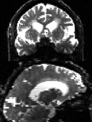
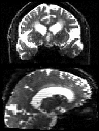
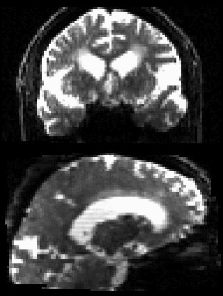
Before and after correction for eddy current-induced distortions.

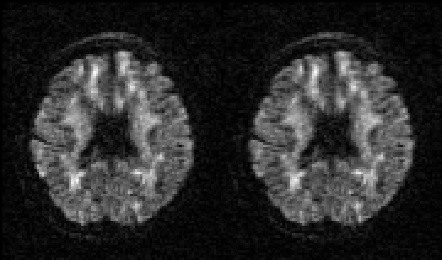Movie of 300 diffusion weighted images acquired as part of the HCP-project before (left panel) and after (right panel) correction of eddy current-induced distortions. N.B. that in the HCP project the phase encode-direction was chosen to be in the x-direction (left-right) instead of in the y-directions (anterior-posterior), which is the more common choice.

What are "eddy current-induced distortions"?

EPI images are very sensitive even to very small off-resonance fields (please see the topup documentation for an explanation of the term "off-resonance field", and why EPI images are affected by it). An off-resonance field can be caused by the object (head) itself disrupting the main magnetic field, as explained in the topup documentation, but is can also be caused by unwanted "eddy" currents (EC) in conductive parts of the scanner gantry. These currents gives rise to a magnetic field, hence the term "eddy current-induced off-resonance field". Any rapidly changing magnetic field will induce currents in conductive materials, and the switching of the gradients in an MR-scanner is precisely such a "rapidly changing magnetic field".

Any EPI acquistion is in principle affected since the image encoding gradient switching will induce eddy currents, but in practice these are quite small and possible to deal with as part of the sequence design. Hence it is mainly a problem for diffusion imaging where the very strong diffusion encoding gradients causes an eddy current-induced field that persist into the image encoding, leading to image distortions. These EC-induced fields tend to be of relatively low spatial order, largely resembling the diffusion gradient that preceeded it.

Examples of EC-induced field and distorted images.

The top row shows six diffusion weighted images acquired with diffusion gradients along the direction indicated by the arrows below. Careful visual inspection shows that they are all distorted relative to each other. The off-resonance fields estimated by eddy are shown in the row below, scaled to -60--60 Hz. It can be seen that the estimated fields are to a first approximation a linear field along the direction of the diffusion gradient.

Unlike the susceptibility-induced off-resonance field the EC-induced fields are different for each diffusion direction/volume, which means that unless corrected a given voxel will correspond to different anatomical locations in different volumes (this is what can be seen in the movie above. That is of course a problem for any voxel-wise modelling of the diffusion signal, and needs to be corrected before that stage.

How does `eddy` solve that?

eddy is based on "image registration", i.e. it will align each individual image to a "target" that is not distorted. In general, the alignment (registration) is performed by applying different "undistorting" transforms to the individual image and calculating a cost-function between that and the target. The cost-function is designed in to have a maximum/minimum when the two images are maximally similar. The "undistorting" transform that yields that maximum/minimum is deemed to be the one that undistorts the image to its "true" shape. However, registration of diffusion weighted images can be challenging because the different diffusion images can have very different contrast to each other, especially for high $b$-value data. All the different diffusion weighted images will also have very different contrasts to the $b=0$ image(s). Hence, it is non-trivial to find a suitable cost-function, and also to find a suitable, undistorted target image. eddy solves this by using a Gaussian Process to make a prediction about what the individual image "should" look like based on all the other images. That way the contrast of the target image will be the same as the image we want to align, and the target image will be in undistorted space if data has been acquired on the whole-sphere or in a less distorted space if it has been acquired on the half-sphere (see below for a discussion about whole- vs half-sphere). A schematic of the process can be seen below.

Schematic of how eddy works.

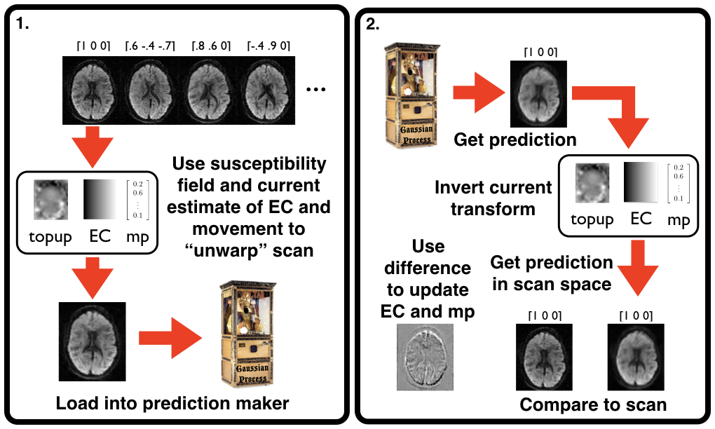The eddy registration can be thought of as two steps. 1. The loading step in which the current estimates of EC field, subject movement etc are applied to all the image volumes before being loaded into a Gaussian Process. And 2. The estimation step where a prediction is made for each image volume, the current estimates of correction are "undone" and the resulting image is compared to the observed scan for that diffusion gradient. The difference between the two is what drives the registration. These two steps together comprise one iteration, and `eddy` is typically run for five to ten such iterations.

The following is a more detailed look at some of the steps involved, and the additional artefacts that eddy is able to correct.

The Gaussian Process

The Gaussian Process is simply a way to describe the data based on very few and general assumptions. These assumptions are - the signal from two acquisitions acquired with diffusion weighting along two vectors with a small angle between them is more similar than for two acquisitions with a large angle between them - the signal from two acquisitions along vectors v and -v is identical.

From these two assumptions it also follows that: - if v1 and v2 are two vectors with a "small" angle between them so that it can be assumed that the signal from the corresponding acquisitions is "similar" then v1 and -v2 are equally similar. It is able to model signals that doesn't conform to the simple diffusion tensor, while at the same time being very fast to calculate due to it being a linear model.

Gaussian Process fit to multi-shell data.

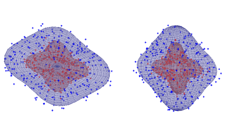The figure shows data-points from a $b=1000$ shell (blue points) and a $b=3000$ shell (red points) from a voxel with a three-fibre crossing. For a given point, the distance from the centre shows the image intensity and the direction shows the diffusion gradient direction for the pertinent volume. The Gaussian Process fit is shown as a blue mesh for the $b=1000$ and a red for the $b=3000$ shell. It can be seen how well the Gaussian Process is able to model the rather complex signal in this voxel.

What data does eddy need?

There are very few restrictions on the data for running eddy. This is somewhat contrary to what some believe, which is probably due to an unfortunate formulation in a previous version of the online documentation. So, to be very clear: - eddy does not need data to have been acquired on the whole-sphere. - eddy does not need data to have been acquired with opposing PE-direction for all directions.

Having said that, it is helpful if data is acquired on the whole-sphere, and it will now be explained why. And also what needs to be done if is is not. So, first of all:

What is meant by whole- vs half-sphere?

When acquiring diffusion data one typically wants to sample the diffusion sphere as evenly as possible, i.e. one wants one's diffusion directions to be as evenly distributed as possible. This is so as to minimise any directional bias in the modelling of the diffusion signal (i.e. we do not want to be biased against a fibre going in a specific direction because we haven't measured the signal in that direction). It is not anything specific to pre-processing or eddy.
However, the diffusion signal is rotationally symmetric, i.e. the signal is identical for the diffusion gradients $\mathbf{v}$ and $-\mathbf{v}$ so it is not strictly speaking neccessary to sample on the whole sphere. It is therefore common to consider for example only diffusion vectors with a positive $z$-component, because for every diffusion vector $\mathbf{v}$ with a positive $z$-component we have de facto also "measured" $-\mathbf{v}$ which has a negative $z$-component.

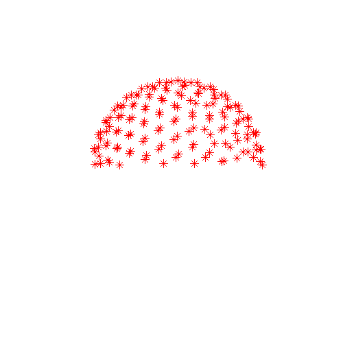
Data sampled on the half-sphere	Data sampled on the whole-sphere

The red dots corresponds to sample points on the diffusion sphere, i.e. they can be thought of as endpoints of a set of arrows starting at the origin and representing the diffusion gradients. The whole sphere on the right has been created by negating a subset of the vectors on the left. Hence they are identical w.r.t. sampling the diffusion signal.

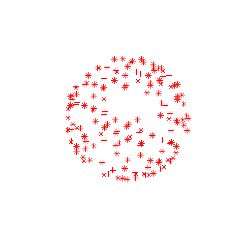
If you are not sure of how your data was acquired you can use this matlab code to visulalise the directions:

bvecs = load('bvecs'); % Assuming your filename is bvecs
figure('position',[100 100 500 500]);
plot3(bvecs(1,:),bvecs(2,:),bvecs(3,:),'*r');
axis([-1 1 -1 1 -1 1]);
axis vis3d;
rotate3d

The final command (rotate3d) will allow you to use the pointer to rotate the plot which is essential as from some angles a half sphere looks just like a whole sphere.

Why is it helpful to `eddy` if data is sampled on the whole-sphere?

The reason that it works to use a Gaussian Process prediction as a target for the registration is that it will be in undistorted space if data has been sampled on the whole-sphere. The prediction is a weighted average of all the other images, and all of those images will be distorted in different ways. The eddy currents are caused by the preceeding diffusion gradients and if plotting the EC-parameters against the different components ($x$, $y$ and $z$) of the they show a clear, typically linear, relationship with the origin indicating that when the gradient component is zero the EC-parameter is zero (see the figure below).
What that means is that when a gradient has a zero component for a given direction ($x$, $y$ or $z$), then there is none of the EC associated with that particular component. That sounds like quite a trivial statement, but importantly what it also means is that for a collection of volumes acquired with different diffusion gradients the average distortion associated with a given gradient component will be zero as long as the average of that component across all volumes is zero. And that is of course the case for data acquired on the whole sphere. I.e. the Gaussian Process prediction (the target for the registration) will be in undistorted space, and the images will be immediately registered into undistorted space.
If, in contrast, the data has been acquired on the half-sphere there will be a non-zero average of one of the components (often, but not neccessarily, the $z$-component), and hence there will be a non-zero EC from that component. That means that the images will not be registered to a zero distortion space, but rather a space that still has some of the distortions associated with the component that has a non-zero mean. They will still be registered to the same space, so this problem can not be detected by running a movie of the corrected images. It is just that the space is not quite the undistorted space.
This all sounds a little depressing if you didn't acquire your data on the whole-sphere. But please read on, the next section will show that there is a very easy solution that amounts to no more than adding an extra parameter to the eddy command line.

What do we need to do if our data is sampled on the half-sphere?

It is very simple. All you need to do is to add slm=linear to your eddy command line. What that does is to model the EC parameters that eddy has estimated as a linear function of the diffusion gradient components and centres any non-zero offset at the origin. This is, hopefully, better explained by the figure below than I can hope to achieve with words.

Demonstration of unbiasing through second-level modelling.

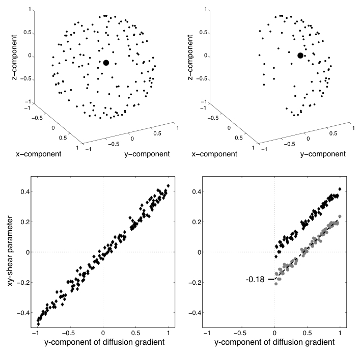The top-left panel shows the sampling points of a data set sampled on the whole sphere. The bottom left panel shows the estimates of one of the EC-parameters (the xy-shear parameter) plotted against the $y$-component of the diffusion gradient. It can be seen that the estimates are quite well described as a linear function of the $y$-component. The top right panel shows the sampling for the same data set, but now after having removed any volumes/directions with a negative z-component. The larger black dot shows the mean/centre-of-gravity of the different directions, and it can be seen that it has a clear non-zero component in the $y$-component. The grey circles in lower right panel shows the xy-shear estimates when eddy was run on the half-sphere data. It can be seen that the zero-point has been shifted since the "average distortion point" in the half-sphere data has a non-zero $y$-component. But by fitting a straight line to these points we get an intercept (in this case -0.18), and by adding that intercept the estimates become almost (you wouldn't expect them to be exactly identical since they only use half the data) identical to the whole-sphere case.

So, again, just to be crystal clear: - eddy does not need data to have been acquired on the whole-sphere. - eddy does not need data to have been acquired with opposing PE-direction for all directions.

What distortion model does eddy use?

The seminal paper by Jezzard el al. describes the distortions as a $yx$-shear, a $y$-zoom and a $z$-translation. This was predicated on the EC-induced field being a linear combination of $x$, $y$ and $z$ linear gradients, the PE-direction being along $y$ and on considering it as a 2D problem. In the figure below is a more general explanantion for how the EC-induced fields translate into distortions.

Explanation of how EC-fields translate into distortions.

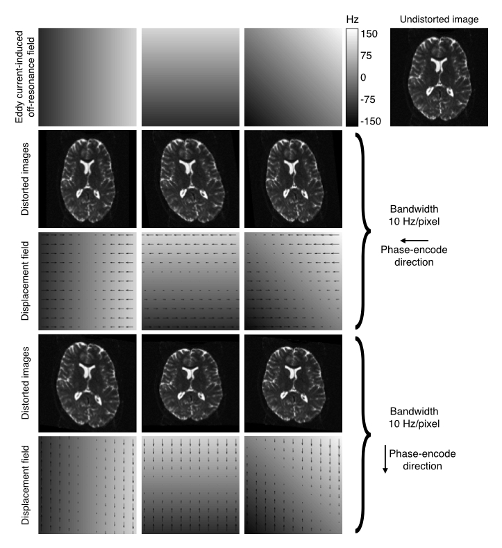The top row shows EC-fields linear in the $x$, $y$ and $xy$-directions in columns 1-3 respectively. The fourth column shows an undistorted image. Row two shows the resulting distorted images for data acquired with the phase-encoding in the $y$-direction, and row three shows the corresponding displacement fields. Rows four and five shows the same for the case where the phase-encoding is in the $y$-direction.

The fields and distortions in the figure above still assume that the EC-fields are "perfect" linear combinations of linear gradients. However, that is not a given and there is ample evidence that this is not generally true (I would personally go as far as to say the it is generally not true). When validating eddy on the HCP data we found strong evidence both for quadratic and cubic terms, even though the cubic terms where sufficiently small to safely ignore even though they could be reliably detected.
Given that not even presumably "linear" fields generated by the gradient coils themselves are particularly linear (and require non-linearity correction to produce high fidelity images), it is hardly surprising that the EC-induced fields are not either. The default in eddy is therefore to model the EC-field as a quadratic, including a constant term, yielding a total of ten parameters per field/volume. It is also possible to specify a linear (4 parameters) or a cubic (20 parameters) field by adding --flm=linear or --flm=cubic respectively to the command line.

What corrections does eddy perfom, apart from for eddy currents?

eddy performs a number of additional corrections:

Inter-volume subject movement
Movement-related signal drop out
Intra-volume subject movement
Susceptibility-by-movement interaction

Inter-volume subject movement

In addition to EC-induced distortions, subjects will inevitably move. So eddy includes a rigid-body subject movement model. This adds an additional six parameters to the transformation model (taking the total to 16 for the quadratic EC-model), which are jointly estimated with the EC-parameters. The estimated rotation parameters are also used to generate a set of rotated bvecs (table of diffusion gradients) that can be used in lieu of the original ones for further processing.

The contrast mechanism of diffusion MR imaging is based on a signal loss that depends on the spins moving along the direction of the diffusion gradient during the diffusion encoding phase of the sequence. So it is not terribly surprising that head movement occurring during the diffusion encoding phase of the sequence can also lead to signal loss. These often manifest as an almost total loss of signal in a slice (or group of slices in the case of multi-band acquisitions). But sometimes as a partial signal loss across an entire slice, or as signal loss in only part of a slice (when it is caused by for example pulsatile movement that only affects part of the slice (e.g. the brain stem)).
eddy can detect these cases by comparing the observed average signal in a slice to the predicted (using the Gaussian Process prediction) signal. And when the difference between the observed and predicted signal falls above some number (4 by default) of standard deviations, it will replace that slice with its prediction. That will ensure that the signal loss doesn't have an impact on eddy's ability to estimate EC/movement or on downstream modelling of the diffusion signal. In order to do this one needs to include --repol on the command line. It is described in more detail here, and we strongly recommend using outlier replacement.

Example of data with and without outlier-replacement.

Movie of two adjacent slices alternating between with and without outlier-replacement when running eddy. The images are in "corrected space", i.e. after having been registered into the space of the first $b=0$ volume. Note how subject movement has meant that the original drop-out slices have been rotated out-of-plane such that they now appear as dark diagonal bands.

Intra-volume subject movement

The slices in an EPI sequence are not all acquired at the same time. It will typically take somewhere between 3 and 8 seconds (depending on if multi-band is used or not) to acquire them all. That means that any sudden movement can result in a "disrupted" stack of slices, i.e. when stacked they no longer constitute a true representation of the volume. In diffusion the slices are typically acquired in an "interleaved" fashion, meaning that all odd slices are acquired first and then all the even slices. That means that subject movement during the acquisition typically leads to a tell-tale zig-zag pattern along the edges of the image.

Explanation of zig-zag pattern from intra-volume movement.

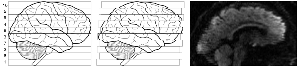The leftmost image shows the outline of a brain, and ten "slices" acquired in the order indicated by the numbers on the left. The middle image shows the same brain, but now there was a continouos translation in the Post->Ant direction. The rightmost image shows an actual MR image displaying the same telltale pattern.

By adding the parameter --mporder=n, where n is a number greater than 0, the eddy command line one can correct also for intra-volume movement. The figure below shows the effects of adding outlier-replacement and intra-volume motion correction to a problematic data set with lots of subject movement.


Original data	After EC and inter-volume motion correction	After EC, inter-volume motion and outlier correction	After EC, intra-volume motion and outlier correction

Susceptibility-by-movement interaction

The susceptibility field, for example as estimated using topup, is strictly speaking only valid for that specific subject location. As a first approximation the susceptibility field "follows the object", i.e. if the subject moves 5 mm to the left after the data for the fieldmap was acquired, the field will stay the same but also move 5 mm to the left. But, that is only a first approximation.
If there are out-of-plane rotations, and most subject movements include those, the field no longer just follow the object, it also changes. These changes are not huge, on the order of ~5 Hz/degree rotation in the most affected areas, compared to ~150 Hz in the off-resonance field in the most affected areas. Even after a rotation of more than 5 degrees the old and the new field "look" very similar. But, nevertheless, 5 degrees can correspond to ~25 Hz, which in turn can correspond to more than two voxels distortion, in the most affected areas. That means that images acquired with the subject in different positions will be differently distorted, and even after alignment they will not match up. eddy is able to estimate how the field changes as a consequence of subject movement. All one needs to do is to include --estimate_move_by_susceptibility on the command line. We recommend using it whenever subject movements are "large". Similarly to inter-volume subject movement above this is often the case with for example children or elderly patients. But it is not limited to "fast" movement, so it is useful for example also when someone relaxes in a break between scans and happens to move as part of that.

Data before and after movement correction and correction for susceptibility-by-movement.

Movie of simulated data of a "subject" that moves a lot. The original images are in the left columne. The middle column shows the same data after correction for movement using eddy. It can be seen that although the gross movement has been corrected, it "looks like" there is still movement of the temporal lobe. This is caused by variable susceptibility distortions in that area. The final column shows the data after correction for movement *and* susceptibility-by-movement correction.

Referencing

The main reference that should be cited when using eddy is

[Andersson 2016a] Jesper L. R. Andersson and Stamatios N. Sotiropoulos. An integrated approach to correction for off-resonance effects and subject movement in diffusion MR imaging. NeuroImage, 125:1063-1078, 2016.

If you use the --repol (replace outliers) option, please also reference

[Andersson 2016b] Jesper L. R. Andersson, Mark S. Graham, Eniko Zsoldos and Stamatios N. Sotiropoulos. Incorporating outlier detection and replacement into a non-parametric framework for movement and distortion correction of diffusion MR images. NeuroImage, 141:556-572, 2016.

If you use the slice-to-volume motion model (accessed by the --mporder option) please also reference

[Andersson 2017] Jesper L. R. Andersson, Mark S. Graham, Ivana Drobnjak, Hui Zhang, Nicola Filippini and Matteo Bastiani. Towards a comprehensive framework for movement and distortion correction of diffusion MR images: Within volume movement. NeuroImage, 152:450-466, 2017.

If you use the susceptibility-by-movement correction in eddy (accessed by the option --estimate_move_by_susceptibility) please also reference

[Andersson 2018] Jesper L. R. Andersson, Mark S. Graham, Ivana Drobnjak, Hui Zhang and Jon Campbell. Susceptibility-induced distortion that varies due to motion: Correction in diffusion MR without acquiring additional data. NeuroImage, 171:277-295, 2018.

You are welcome to integrate eddy in scripts or pipelines that are subsequently made publicly available. In that case, please make it clear that users of that script should reference the paper/papers above.

Other papers of interest

There is a slightly less technical (than in the papers) overview of the principles of eddy and all the functionality implemented up to 2020 in the book chapter

[Andersson 2021] Jesper L. R. Andersson. Diffusion MRI artifact correction. In: Advanced Neuro MR Techniques and Applications. Eds In-Young Choi and Peter Jezzard. Academic Press, 2021.

For those interested in Gaussian Processes, the book by Rasmussen and Williams is an excellent introduction

[Rasmussen 2006] Rasmussen C.E. and Williams C.K.I. Gaussian Processes for Machine Learning. MIT Press, 2006.

and the following paper describes how eddy uses a Gaussian Process to make model-free predictions of what a diffusion weighted image should look like

[Andersson 2015] Jesper L.R. Andersson and Stamatios N. Sotiropoulos. Non-parametric representation and prediction of single- and multi-shell diffusion-weighted MRI data using Gaussian processes. NeuroImage, 122:166-176, 2015.

The following paper compares the performance of eddy to the previous FSL tool eddy_correct

[Graham 2015] Mark S. Graham, Ivana Drobnjak and Hui Zhang. Realistic simulation of artefacts in diffusion MRI for validating post-processing correction techniques. NeuroImage, 125:1079-1094, 2015.

The following paper makes the case for modelling and correcting for how the susceptibility induced field changes with subject movement

[Graham 2017] M.S. Graham, I. Drobnjak, H. Zhang. Quantitative assessment of the susceptibility artefact and its interaction with motion in diffusion MRI. PLoS ONE, 12(10), 2017.