User's guide for eddy
Documentation in progress
We have migrated the FSL documentation from the old Wiki format to markdown. These pages are part of that migration. I think that is is pretty much done now, and much better than the old documentation. But if you prefer to use the old documentation meanwhile it is still available here.
The eddy executables
eddy is a very computationally intense application, so in order to speed things up it has been parallelised. This has been done in two ways, resulting in two different executables
eddy_cpu: This has been parallelised using the C++ threads library, and allowseddyto use more than one CPU core when running. The maximum number of cores used is determined by the--nthr=nparameter, wherenis the desired number of cores. If the user requests more threads than there are hardware cores the number will be restricted to the latter.eddy_cuda: This has been parallelised with CUDA, which allowseddyto use an Nvidia GPU if one is available on the system.
Both of the executables have exactly the same functionality, though eddy_cpu will be noticeably slower unless a very large number of cores are used.
In addition to those there is also a Python script called eddy, which will call one of the executables above depending on if it can detect an Nvidia GPU on the system or not.
In the past there was a need to match the Cuda version of eddy with the version of the Cuda library that was installed on one's machine. That is no longer neccessary. There are still some requirements, but it is very unlikely that you would not fulfill those. See the FAQ section if your are interested in the details.
Running eddy
Over the years eddy has grown in capabilities and complexity, which means that an eddy command line can now look quite intimidating. Here we will introdce you to your first "plain vanilla" eddy command line. The example includes running topup prior to eddy, as this would be the most typical use case.
The data
The data for this example consists of one set of volumes acquired with phase-encoding A>>P consisting of 5 b=0 volumes and 59 diffusion weighted volumes
| `data.nii.gz` |
|---|
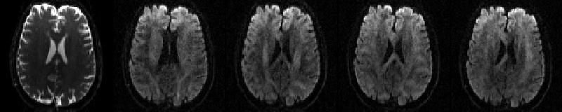 |
| First b=0 volume and the first four dwis of the A>>P data. |
and one single b=0 volume with phase-encoding P>>A.
| `P2A_b0.nii.gz` |
|---|
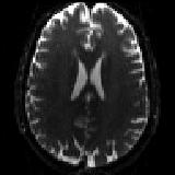 |
| The P>>A data. |
Note how the shape of the b=0 scan is different for the two different acquisitions. This is what topup will use in order to calculate the susceptibility induced off-resonance field.
Running topup on the b=0 volumes
The first thing we do is to run topup to estimate the susceptibility induced off-resonance field. In order to prepare the data for topup we issue the following commands
fslroi data A2P_b0 0 1
fslmerge -t A2P_P2A_b0 A2P_b0 P2A_b0
printf "0 -1 0 0.0646\n0 1 0 0.0646" > acqparams.txt
The first two commands will produce a file called A2P_P2A_b0.nii.gz containing the two b=0 volume, and the third command will create a file (named acqparams.txt) that informs topup/eddy of how the data was collected. This file is described here, here and in more detail here.
Now it is time to run topup which we do with the command
topup --imain=A2P_P2A_b0 --datain=acqparams.txt --config=b02b0.cnf --out=my_topup_results \
--iout=my_hifi_b0
which will give us as our main result two files named my_topup_results_fieldcoef.nii.gz and my_topup_results_movpar.txt. The first of these contains an estimate of the susceptibility induced off-resonance field (or rather the spline coefficients from which it can be generated). The second contains the rigid body movement parameters between the 3D volumes in the 4D file specified as --imain. In the example above we have also specified the optional parameter --iout that results in the additional output my_hifi_b0.nii.gz containing the input images after correction.
Next, Running eddy
Before we can run eddy we need to do a couple of more preparations. First of all we need a mask that separates brain from non-brain. This is no different from for example the mask that dtifit needs. Since eddy will work in a non-distorted space we will base the mask on my_hifi_b0.nii.gz (the secondary output from our topup command above). We generate this mask with the commands
which results in the file my_hifi_b0_brain_mask.nii.gz. It will be a good idea to check this stage to ensure bet has done a good job of extracting the brain.
The final thing we need to do is to create an index file that tells eddy which line/of the lines in the acqparams.txt file that are relevant for the data passed into eddy. In this case all the volumes in data.nii.gz are acquired A->P which means that the first line of acqparams.txt describes the acquisition for all the volume. We specify that by passing a text file with as many ones as there are volumes in data.nii.gz. One way of creating such a file would be to type the following commands
where 64 is the total number of volumes in data.nii.gz and needs to be replaced by the number of volumes in your data.
We are now in a position to run eddy using the command
eddy --imain=data --mask=my_hifi_b0_brain_mask --acqp=acqparams.txt --index=index.txt \
--bvecs=bvecs --bvals=bvals --topup=my_topup_results --out=eddy_corrected_data
eddy with outlier replacement
When (not if) a subject makes a movement that coincides in time with the diffusion encoding part of the sequence, there will be partial or complete signal dropout. The dropout will affect the whole (the most common case) or parts of a slice. In the presence of out-of-plane rotations these slices will turn into diagonal bands when eddy rotates the volume back. If uncorrected this will affect any measures derived from the data. A more in depth explanation can be found here and here.
All that is needed to add outlier replacement to the example above is to add --repol to the command line. If the data was acquired with multi-band (also known as Simultaneous Multi Slice (SMS)) you also need to inform eddy about the multi-bans structure, which you can do with --json=my_json_file.json.
eddy --imain=data --mask=my_hifi_b0_brain_mask --acqp=acqparams.txt --index=index.txt \
--bvecs=bvecs --bvals=bvals --topup=my_topup_results --repol --json=my_json_file.json \
--out=eddy_corrected_data
The exact details of how the outlier replacement is performed can be specified by the user, and in particular if ones data has been acquired with multi-band it can be worth taking a look here.
Correcting slice-to-volume (intra-volume) movement with eddy
A common assumption for movement correction methods is that the subject remains still during the time is takes to acquire a volume (TR, typically 2-8 seconds for diffusion) and that any movement occurs between volumes. This is of course not true, but as long as the movement is slow relative the TR, it is a surprisingly good approximation.
However, for some subjects (for example small children) that assumption no longer holds. The result is a "corrupted" volume where the individual slices no longer stacks up to a "valid" volume. The leads to a telltale zig-zag pattern in a coronal or sagittal view when the slices are acquired in an interleaved fashion (that is the typical way to acquire diffusion data). A more in depth explanation can be found here and here.
So, let us now pretend that our data set suffers from problems with lots of subject movement, including intra-volume movement. The "lots of subject movement part" means that we might need to make eddy more robust to large initial differences in location. We can do that by running more iterations, and also by smoothing the data for the first iterations (N.B. that this does not affect the smoothness of the output). That is done by adding for example --niter=8 and --fwhm=10,8,4,2,0,0,0,0.
Then we need to tell eddy to also run slice-to-volume registration, which we do by adding the parameter --mporder=n, where n is some integer greater than 0. There is an in-depth description of --mporder here, but as a general rule we recommend setting it to somewhere in the interval \(N_{sl}/8\) to \(N_{sl}/2\), where \(N_{sl}\) is the number of slices in your data. Our data has 64 slices, so we set --mporder=16.
eddy --imain=data --mask=my_hifi_b0_brain_mask --acqp=acqparams.txt --index=index.txt \
--bvecs=bvecs --bvals=bvals --topup=my_topup_results --niter=8 --fwhm=10,8,4,2,0,0,0,0 \
--repol --json=my_json_file.json --out=eddy_corrected_data --mporder=16
N.B. that for multi-band data we need to supply the multi-band structure also for slice-to-volume registration. But in this case we added it already for the outlier replacement.
Correcting susceptibility-by-movement interactions with eddy
The off-resonance field that is caused by the subject head itself disrupting the main field in the scanner is referred to as the susceptibility induced field. This is the field that we estimate from blip-up-blip-down data using topup, or measure using a dual echo-time gradient echo sequence.
If/when the subject moves the field will, as a first approximation, move with the subject. To make it concrete, let us say we acquired blip-up-blip-down data and estimated the field with the subject in one location, and that the subject subsequently move 5mm in the z-direction. To a first approximation the new field is identical to the measured field, but translated 5mm in the z-direction.
However, if the movement includes a rotation around an axis that is non-parallel to the magnetic flux (z-axis) the field will change such that it is no longer sufficient to rotate the measured field to the new position. There is an option in eddy to estimate how the field changes as the subject moves. It uses, as default, a first order Taylor expansion with respect to pitch and roll (rotation around \(x\) and \(y\)). More detail can be found here and here.
All we need to do in order to add this to our eddy run is to add --estimate_move_by_susceptibility. Hence, our eddy command line now becomes
eddy --imain=data --mask=my_hifi_b0_brain_mask --acqp=acqparams.txt --index=index.txt \
--bvecs=bvecs --bvals=bvals --topup=my_topup_results --niter=8 --fwhm=10,8,4,2,0,0,0,0 \
--repol --json=my_json_file.json --out=eddy_corrected_data --mporder=16 \
--estimate_move_by_susceptibility
And that is pretty much as advanced as it ever gets with eddy.
Understanding eddy output
The --out parameter specifies the basename for all output files of eddy. It is used as the name for all eddy output files, but with different extensions.
| :warning: Work in progress |
|:----------------------------|
There is currently (April 2024) a re-write in process so that in the future eddy will stop writing multiple text-files, and instead output a single .json file which will subsume all the text-files, and also offer much more detailed information of how eddy was run. If you are using a recent version of eddy you will already have seen .json output files. However, at the present time the format is still in flux. When we have completed the change to a .json file there will still be the option to write the "old style" output described below.
In the following we assume that user specified --out=my_eddy_output.
Files that are always written
-
my_eddy_output.nii.gz
This is the main output and consists of the input data after correction for eddy currents and subject movement, and for susceptibility if--topupor--fieldwas specified. It may also have been corrected for signal dropout, intra-volume movement and susceptibility-by-movement interaction depending on if--repol,--mporderand--estimate_move_by_susceptibilitywere set. Chances are this is the only output file you will be interested in (in the context ofeddy). -
my_eddy_output.eddy_parameters
This is a text file with one row for each volume in--imainand one column for each parameter. The first six columns correspond to subject movement starting with three translations followed by three rotations. The remaining columns pertain to the EC-induced fields and the number and interpretation of them will depend of which EC model was specified. -
my_eddy_output.eddy_rotated_bvecs
When a subject moves such that it constitutes a rotation around some axis and this is subsequently reoriented, it will create an inconsistency in the relationship between the data and the "bvecs" (directions of diffusion weighting). This can be remedied by using themy_eddy_output.eddy_rotated_bvecsfile for subsequent analysis. For the rotation to work correctly the bvecs need to be "correct" for FSL before being fed intoeddy. The easiest way to check that this is the case for your data is to run FDT and display the_V1files infslvieworFSLeyesto make sure that the eigenvectors line up across voxels.my_eddy_output.eddy_rotated_bvecs_for_SLR
Is generated when--resamp=lsris specified. When performing a "least-squares reconstruction" each pair (with the same diffusion gradient) of input images is combined into a single corrected output images. That means that the--bvecsfile should contain only half as many diffusion gradient as the original file. The.eddy_rotated_bvecs_for_SLRis generated by rotating the individual gradients within the pair and taking the geometric average of the two.
-
my_eddy_output.eddy_command_txtandmy_eddy_output.eddy_values_of_all_input_parameters
These are files that "document" howeddywas run on a given data set (though there is no formal link to the other output files apart from the name)..eddy_command_txt
Is a copy of theeddycommand line..eddy_values_of_all_input_parameters
Is a list of the values of all the parameters that was used byeddy. These include also all the parameters that weren't explicitly set on the command line.
-
my_eddy_output.eddy_movement_rms
A summary of the "total movement" in each volume is created by calculating the displacement of each voxel and then averaging the squares of those displacements across all intracerebral voxels (as determined by --mask) and finally taking the square root of that. The file has two columns where the first contains the RMS movement relative the first volume and the second column the RMS relative the previous volume. -
my_eddy_output.eddy_restricted_movement_rms
There is an inherent ambiguity between any EC component that has a non-zero mean across the FOV and subject movement (translation) in the PE direction. They will affect the data in identical (or close to identical if a susceptibility field is specified) ways. That means that both these parameters are estimated by eddy with large uncertainty. This doesn't matter for the correction of the images, it makes no difference if we estimate a large constant EC components and small movement or if we estimate a small EC component and large movement. The corrected images will be (close to) identical. But it matters if one wants to know how much the subject moved. We therefore supplies this file that estimates the movement RMS as above, but which disregards translation in the PE direction. -
my_eddy_output.eddy_post_eddy_shell_alignment_parameters
This is a text file with the rigid body movement parameters between the different shells as estimated by a mutual information based registration (see--dont_peasfor details). These parameters will be estimated even if--dont_peashas been set, but in that case they have not been applied to the corrected images inmy_eddy_output.nii.gz. -
my_eddy_output.eddy_post_eddy_shell_PE_translation_parameters
This is a text file with the translation along the PE-direction between the different shells as estimated by a post-hoc mutual information based registration (see--dont_sep_offs_movefor details). These parameters will be estimated even if--dont_sep_offs_movehas been set, but in that case they have not been applied to the corrected images inmy_eddy_output.nii.gz. -
my_eddy_output.eddy_outlier_report
This is a text-file with a plain language report on what outlier slices eddy has found. This file is always created, as are the other my_eddy_output.eddy_outlier_* files described below, even if the--repolflag has not been set. Internally eddy will always detect and replace outliers to make sure they don't affect the estimation of EC/movement, and if--repolhas not been set it will re-introduce the original slices before writingmy_eddy_output.nii.gz. -
my_eddy_output.eddy_outlier_map,my_eddy_output.eddy_outlier_n_stdev_mapandmy_eddy_output.eddy_outlier_n_sqr_stdev_map
These are numeric matrices in ASCII format that all have the same general layout. They consist of an initial line of text, after which there is one row for each volume and one column for each slice. Each row corresponding to a b=0 volume is all zeros since eddy don't consider outliers in these. The meaning of the numbers is different for the three files.-
.eddy_outlier_map
All numbers are either 0, meaning that scan-slice is not an outliers, or 1 meaning that is is. -
.eddy_outlier_n_stdev_map
The numbers denote how many standard deviations off the mean difference between observation and prediction is. -
.eddy_outlier_n_sqr_stdev_map
The numbers denote how many standard deviations off the square root of the mean squared difference between observation and prediction is.
-
File that is only written if the --repol flag was set.
my_eddy_output.eddy_outlier_free_data.nii.gz
This is the original data given by --imain not corrected for susceptibility or EC-induced distortions or subject movement, but with outlier slices replaced by the Gaussian Process predictions. This file is generated for anyone who might want to use eddy for outlier correction but who want to use some other method to correct for distortions and movement. Though why anyone would want to do that is not clear to us.
File that is only written if the --mporder option has been set to a value greater than zero.
my_eddy_output.eddy_movement_over_time
This is a text files with one row of six values for each excitation. The values in a row are translation (mm) in the x-, y- and z-directions followed by rotations (radians) around the x-, y- and z-axes. If one for example has a data set of 36 volumes with 66 slices each and an MB-factor (Multi Band) of 2 the.eddy_movement_over_timefile will have 36*66/2=1188 lines.
File that is only written if the --estimate_move_by_susceptibility was set.
my_eddy_output.eddy_mbs_first_order_fields.nii.gz
This is a 4D image file containing the partial derivative fields with respect to pitch (rotation around the \(x\)-axis) and roll (rotation around the \(y\)-axis).
Other files only written if the corresponding flags are set.
-
my_eddy_output.eddy_cnr_maps
Written if--cnr_mapsis set. This is a 4D image file with N+1 volumes where N is the number of non-zero b-value shells. The first volume contains the voxelwise SNR for the b=0 shell and the remaining volumes contain the voxelwise CNR (Contrast to Noise Ratio) for the non-zero b-shells in order of ascending b-value. For example if your data consists of 5 b=0, 48 b=1000 and 64 b=2000 volumes,my_eddy_output.eddy_cnr_mapswill have three volumes where the first is the SNR for the b=0 volumes, followed by CNR maps for b=1000 and b=2000. The SNR for the b=0 shell is defined as mean(b0)/std(b0). The CNR for the DWI shells is defined as std(GP)/std(res) where std is the standard deviation of the Gaussian Process (GP) predictions and std(res) is the standard deviation of the residuals (the difference between the observations and the GP predictions). Themy_eddy_output.eddy_cnr_mapscan be useful for assessing the overall quality of the data. -
my_eddy_output.eddy_residuals
Written if--residualsis set. This is a 4D image file with the same number of volumes as the input (--imain) data. The order of the volumes is the same as for the input data and each voxel contains the difference between the observation and the prediction.
Categorised list of parameters
Parameters that specify input files
-
--imain=filename
Name of a file with input images. E.g.all_my_images.nii. Compulsory. -
--mask=filename
Name of a file with mask specifying brain vs no-brain. E.g.my_brain_mask.nii. Compulsory. -
--acqp=filename
Name of text file with information about the acquisition of the images in--imain. E.g.my_scan_pars.txt. Compulsory. -
--index=filename
Name of text file specifying the relationship between the images in--imainand the information in--acqpand--topup. E.g.index.txt. Compulsory. -
--bvecs=filename
Name of text-file with normalised diffusion gradients. Compulsory. -
--bvals=filename
Name of text-file with b-values. Compulsory.--b_range
Determines maximum range of b-values within the shells.
-
--topup=basename
Name of output from a previous topup run. Should be the same as the argument given to topup's--out. Optional. -
--json=filenameor--slspec=filename
Text-files describing slice acquisition order. Mutually exclusive and semi-optional. They are neccessary if for example performing intra-volume motion correction, or if performing outlier-replacement with--ol_type=gwor--ol_type=both.--json=filename
.json file produced by Dicom to Nifti converter, for exampledcm2niix. It is strongly recommended to use a--jsonfile instead of an--slspecfile.--slspec=filename
Bespoke text file specifying slice acquisition order.
-
--field=filename
Name of image volume representing the susceptibility field. Should be in Hz. Optional.--field_mat=filename
Name of rigid body matrix specifying the relative positions of--fieldand--imain. Optional.
Parameter specifying names of output-files
--out=basename
Basename for output-files. The corrected images will be named"basename".nii.gz. Other output files will be named"basename".eddy_*where the * specifies the specific type of output. Compulsory.
Parameters specifying how eddy should be run
-
--flm=linear/quadratic/cubic
Spatial model for the field generated by eddy currents. Default quadratic. -
--slm=none/linear/quadratic
Model for how diffusion gradients generate eddy currents. Default none. -
--fwhm="fwhm in mm"
Filter width to use for pre-filtering of data for the estimation process. Default 0. -
--niter="required number of iterations"
Specifies how many iterations should be run. Default 5. -
--interp=spline/trilinear
Specifies interpolation model during estimation. Default spline. -
--resamp=jac/lsr
Specifies final resampling strategy. Default jac.--fep
Fill Empty Planes. Default false. Only meaningful in conjunction with--resamp=lsr. Interpolates across any "empty planes" orthogonal to the phase-encode direction. It is unclear why they are there (empty), but for many vendors/sequences they are.
-
--nvoxhp="number of voxels"
Specifies number of voxels to use for GP hyperparameter estimation. Default 1000. -
--ff="number between 1 and 10"
Fudge factor that imposes Q-space smoothing during estimation. Default 10. -
--dont_sep_offs_move
Do not attempt to separate subject movement from field DC component. Default false. -
--dont_peas
Do not end with an alignment of shells to each other. Default false.
Parameters pertaining to outlier replacement
-
--repol
Replace outliers. Default false. Likely to become default, and parameter deprecated soon. -
--ol_nstd="number of standard deviations"
Number of standard deviations away a slice must be to qualify as an outlier. Default 4. -
--ol_nvox="number of voxels"
The minimum number of intracerebral voxels in a slice to consider it as an outlier. Default 250. -
--ol_type=sw/gw/both
Base outlier detection on slices (sw) multi-band groups (gw) or both (both). Default sw. -
--ol_ss=sw/pooled
Calculate outlier statistics separately for different shells (sw) or pooled across shells (pooled). Default sw. -
--ol_pos
Consider both positive and negative outliers. Default false. -
--ol_sqr
Consider outliers in sum-of-squared distribution. Default false. -
--mb="multi-band factor"
Specifies multi-band factor (number of simultaneous slices). Default 1. Likely to be deprecated soon.
Parameters pertaining to intra-volume (slice-to-vol) movement correction
-
--mporder="number of basis functions"
Temporal order of movement. Default 0. -
--s2v_niter="number of iterations"
Number of iterations for estimating slice-to-vol movement. Default 5, if--mporder> 0. -
--s2v_lambda="weight of regularisation"Strength of temporal regularisation of slice-to-vol movement. Default 1. -
--s2v_interp=trilinear/splineInterpolation model for estimation of slice-to-vol movement. Default 'trilinear'.
Parameters pertaining to susceptibility-by-movement correction
-
--estimate_move_by_susceptibilityWhen specified eddy estimates how the susceptibility field changes with subject movement. Default false. -
--mbs_niter="number of iterations"Number of iterations for susceptibility-by-movement estimation. Default 10. -
--mbs_lambda="weight of regularisation"Specifies the balance between data and smoothness for the susceptibility rate-of-change fields. Default 10. -
--mbs_ksp="knot spacing in mm"Specifies the spline knot-spacing of the susceptibility rate-of-change fields. Default 10 (mm).
Miscellaneous parameters
-
--cnr_maps
Specifies that shell-wise CNR maps shall be written. Default false. -
--residuals
Specifies that a full 4D data set of residuals shall be written. Default false. -
--data_is_shelled
Do not check that data is shelled. Trust the user. Default false. -
--nthr="Number of CPU threads"
Specifies the number of CPU threads thateddyshould use. It is only relevant for the CPU version. -
--verbose
Print progress information to the screen while running. Can be useful to pipe into file before reporting problems -
--very_verbose
Print very rich progress information to the screen while running. Can be useful to pipe into file before reporting problems -
--help
Take a wild stab.
Commonly used parameters explained
Parameters specifying input files
--imain=filename
Should specify a 4D image file with all your images acquired as part of a diffusion protocol. I.e. it should contain both your dwis and your b=0 images. If you have collected your data with reversed phase-encode blips, data for both blip-directions should be in this file. If you have acquired your data over multiple runs (but with the subject remaining in the scanner) they should be concatenated into one file.
--mask=filename
Single volume image file with ones and zeros specifying brain (one) and no-brain (zero). Typically obtained by running BET on the average of the volumes in the --iout output of topup. If, for whatever reason, you have not previously run topup on your data we suggest you run BET on the first volume b0 volume of your --imain input.
--acqp=filename
A text-file describing the acquisition parameters for the different images in --imain. The format of this file is identical to that used by topup (note that this parameter is also called --datain there) and described in detail here and here.
--index=filename
A text-file that determines the relationship between on the one hand the images in --imain and on the other hand the acquisition parameters in --acqp and (optionally) the subject movement information in --topup. It should be a single column (or row) with one entry per volume in --imain. We will use a small (simplified) example to make it clear.
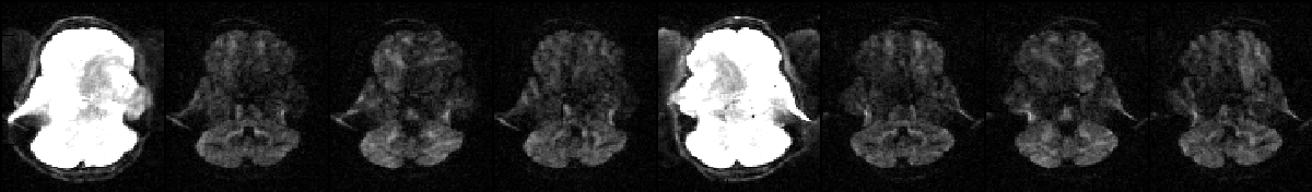
The image above shows a selected slice from each of the eight volumes in --imain. The associated --acqp file is
--imain were acquired using the acquisition parameters on the first row (index 1) of the --acqp file, and that volumes 5--8 were acquired according to the second row (index 2).
--bvecs=filename
A text file with normalised vectors describing the direction of the diffusion weighting. This is the same file that you would use for FDT.
--bvals=filename
A text file with b-values, describing the "amount of" diffusion weighting. This is the same file that you would use for FDT.
- --b_range="max range of b-values within shell"
eddy needs to be able to divide the data into shells, i.e. sets of volumes that have all been acquired with the same b-value. That is complicated by the fact that some manufacturers/sequences will calculate also the "incidental" diffusion weighting from the image encoding gradients and add that to the b-values. Hence it is not enough to sort the volumes on identical b-values. The default --b_range is 50, which means that b-values that fall within a range of 50 will all be included in the same shell. If the range of b-values in your data is greater than that you may need to set it to a higher value. Conversely, if you have several low b-value shell with a small separation you might need to use a lowe value.
--topup=basename
This should only be specified if you have previously run topup on your data and should be the same name that you gave as an argument to the --out parameter when you ran topup.
--json=filename or --slspec=filename
These are two different options for specifying how the slices/MB-groups were acquired.
- --json=filename
Specifies a .json file created for example by dcm2niix as part of the DICOM to Nifti conversion. That file is likely (it depends on the scanner vendor) to contain detailed information about the exact time at which each slice were acquired. If this file is available, and contain slice timing information, we strongly recommend using it since it will help avoid any mistakes. If your .json file contains the attribute "SliceTiming" it most likely has the correct information.
- --slspec=filename
Specifies a text-file that describes how the slices/MB-groups were acquired. This information is necessary for eddy to know how a temporally continuous movement translates into location of individual slices/MB-groups. Let us say a given acquisition has N slices and that m is the MB-factor (also known as Simultaneous Multi-Slice (SMS)). Then the file pointed to be --slspec will have N/m rows and m columns. Let us for example assume that we have a data-set which has been acquired with an MB-factor of 3, 15 slices and interleaved slice order. The file would then be
--json option instead.
--field=filename
If there is no topup output available for your study you may alternatively use a "traditional" fieldmap in its place. This can for example be a dual echo-time fieldmap that has been prepared using PRELUDE. Note that in contrast to for example FUGUE it expects the fieldmap to be scaled in Hz. For boring reasons the filename has to be given without an extension. For example --field=my_field, not --field=my_field.nii.gz.
| :warning: We do not recommend using the --field option | |:--------------------------------------------------------| There are several important caveats with --field, which is why we strongly recommend using a topup derived field if at all possible. These are
- If one uses the same
--acqpfile for both topup and eddy it doesn't matter if one get the total acquisition time or the PE-polarity wrong. The errors in topup and eddy will cancel out and the end results will still be correct. - If the first volume input to topup is the same as the first volume in
--imaintoeddy, the fieldmap will automatically be in the reference space ofeddy. I.e. it will be in perfect alignment with the data it is used to correct. When using the--fieldoption the user is responsible for making sure the fieldmap is registered to the eddy data. eddyassumes that the resulting displacement field (the off-resonance field is a scaled displacement field) i invertible (that it doesn't fold back on itself). Because of the way thatFUGUEdeals with the edges of the fieldmap that is often not the case for fieldmaps processed with FSL. One option in such a case is to instead use the SPM fieldmap toolbox to process the fieldmap.
Another option for avoiding to use the --field option is to use the Synb0-DISCO, which is a toolbox that can synthesize a distortion free b=0 volume from a structural scan (i.e. a T1-weighted scan). The synthetic b=0 volume can then be used together with a b=0 volume from the diffusion data set to run topup.
- --field_mat=filename
Specifies a flirt style rigid body matrix that specifies the relative locations of the field specified by--fieldand the first volume in the file specified by --imain. Ifmy_fieldis the field specified by--field,my_imais the first volume of--imainandmy_matis the matrix specified by--field_mat. Then the commandflirt -ref my_ima -in my_field -init my_mat -applyxfmshould be the command that putsmy_fieldin the space ofmy_ima.
Parameter specifying names of output-files
--out=basename
Specifies the basename of the output. Let us say --out="basename". The output will then consist of a 4D image file named <basename>.nii.gz containing all the corrected volumes and a text-file named <basename>.eddy_parameters with parameters defining the field and movement for each scan and several other files starting with "basename".
Parameters specifying how eddy should be run
--flm=linear/quadratic/cubic
This parameter takes the values linear, quadratic or cubic. It specifies how "complicated" we believe the eddy current-induced fields may be.
Setting it to linear implies that we think that the field caused be eddy currents will be some combination of linear gradients in the \(x\)-, \(y\)- and \(z\)-directions. It is this model that is the basis for the claim "eddy current distortions is a combination of shears, a zoom and a translation". It is interesting (and surprising) how successful this model has been in describing (and correcting) eddy current distortions since not even the fields we intend to be linear (i.e. our gradients) are particularly linear on modern scanners.
The next model in order of "complication" is quadratic which assumes that the eddy current induced field can be modelled as some combination of linear and quadratic terms (\(x\), \(y\), \(z\), \(x^2\), \(y^2\), \(z^2\), \(xy\), \(xz\) and \(yz\)). This is almost certainly also a vast oversimplification but our practical experience has been that this model successfully corrects for example the HCP data (which is not well corrected by the linear model).
The final model is cubic which in addition to the terms in the quadratic model also has cubic terms (\(x^3\), \(x^2y\), etc). We have yet to find a data set where the cubic model performs meaningfully better than the quadratic one. Note also that the more complicated the model the longer will eddy take to run.
--slm=none/linear/quadratic
"Second level model" that specifies the mathematical form for how the diffusion gradients cause eddy currents. For high quality data with 60 directions, or more, sampled on the whole sphere we have not found any advantage of performing second level modelling. Hence our recommendation for such data is to use none, and that is also the default.
If the data has quite few directions and/or is has not been sampled on the whole sphere it can be advantageous to specify --slm=linear.
--fwhm="fwhm in mm"
Specifies the FWHM of a gaussian filter that is used to pre-condition the data before using it to estimate the distortions. In general the accuracy of the correction is not strongly dependent on the FWHM. Empirical tests have shown that ~1-2mm might be best, but by so little that the default has been left at 0.
One exception is when there is substantial subject movement, which may mean that eddy fails to converge in 5 iterations if run with fwhm=0. In such cases we have found that --fwhm=10,0,0,0,0, works well. It means that the first iteration is run with a FWHM of 10mm, which helps that algorithm to take a big step towards the true solution. The remaining iterations are run with a FWHM of 0mm, which offers high accuracy. Another schedule we have used successfully on subjects who move a lot is --niter=8 --fwhm=10,8,4,2,0,0,0,0.
--niter="number of iterations"
eddy does not check for convergence. Instead it runs a fixed number of iterations given by --niter. This is not unusual for registration algorithms where each iteration is expensive (i.e. takes long time). Instead we run it for a fixed number of iterations, 5 as default.
If, on visual inspection, one finds residual movement or EC-induced distortions it is possible that eddy has not fully converged. In that case we primarily recommend that one uses --fwhm=10,0,0,0,0, as described above, to speed up convergence. If that too fails we recommend increasing the number of iterations to something like --niter=8 --fwhm=10,8,4,2,0,0,0,0.
--interp=spline/trilinear
Specifies the interpolation model used during the estimation phase, and during the final resampling if --resamp=jac is used. We strongly recommend spline, which is also the default.
--resamp=jac/lsr
Specifies how the final resampling is performed. The options are
jac: Stands for Jacobian modulation. This is a "traditional" type of interpolation (spline or trilinear depending on the --interp parameter) combined with Jacobian modulation to account for signal pile-up/dilution caused by local stretching/compression. However, in areas of compression (resulting in signal pile-up) there is a loss of resolution that this type of resampling cannot resolve. If acquisitions have not been repeated with opposed PE-directions, this is the only option that can be used.-
lsr: Stands for Least-Squares Reconstruction. This method attempts to use the complimentary information in images acquired with opposing PE-directions, where a compressed area in one of the images will be stretched in the other image. This method can only be used if all acquisitions have been repeated with opposing PE-directions. -
--fep
Stands for "Fill Empty Planes" and is only relevant when--resamp=lsr. For reasons that are not completely clear to us the reconstructed EPI images from some manufacturers contain one or more empty "planes". A "plane" in this context do not necessarily mean a "slice". Instead it can be for example the "plane" that constitutes the last voxel along the PE-direction for each "PE-direction column". The presence/absence of these "empty planes" seems to depend on the exact details of image encoding part of the sequence.
IF --fep is set eddy will attempt to identify the empty planes and "fill them in". The filling will consist of duplicating the previous plane if the plane is perpendicular to the frequency-encode direction and by interpolation between the previous and the "wrap-around plane" if the plane is perpendicular to the PE-direction .
--nvoxhp="number of voxels"
Specifies how many (randomly selected within the brain mask) voxels that are used when estimating the hyperparameters of the Gaussian Process used to make predictions. The default is 1000 voxels, and that is more than sufficient for typical data with resolution of 2x2x2mm or lower. For very high resolution data, such as for example the HCP 7T data, with relatively low voxel-wise SNR one may need to increase this number. The only "adverse" effect of increasing this number is an increase in execution time.
--ff="number between 1 and 10"
This should be a number between 1 and 10 and determines the level of Q-space smoothing that is used by the prediction maker during the estimation of the movement/distortions. Empirical testing has indicated that any number above 5 gives best results. We have set the default to 10 to be on the safe side.
--dont_sep_offs_move
All our models for the EC-field contains a component that is constant across the field and that results in a translation of the object in the PE-direction. Depending on how the data has been acquired it can be more or less difficult to distinguish between this constant component and subject movement. It matters because it affects how the diffusion weighted images are aligned with the b=0 images. Therefore eddy attempts to distinguish the two by fitting a second level model to the estimated constant component, and everything that is not explained by that model will be attributed to subject movement. As of release 5.0.11 it will also perform a Mutual Information based alignment along the PE-direction.
If you set this flag eddy will not do that estimation. The option to turn this off is a remnant from when we did not know how well it would work and it is very unlikely you will ever use this flag. It will eventually be deprecated.
--dont_peas
The motion correction within eddy has greatest precision within a shell and has a bigger uncertainty between shells. There is no estimation of movement between the first b=0 volume and the first diffusion weighted volume. Instead is is assumed that these have been acquired very close in time and that there were no movement between them.
If there are multiple shells or if the assumption of no movement between the first b=0 and the first diffusion weighted volume is not fulfilled it can be advantageous to perform a "Post Eddy Alignment of Shells" (peas). Our testing indicates that the peas has an accuracy of ~0.2-0.3mm, i.e. it is associated with some uncertainty. This precision is still such that peas is performed as default.
But, if one has a data set with a single shell (i.e. a single non-zero shell) and the assumption of no movement between the first b=0 and the first diffusion weighted image is true it can be better to avoid that uncertainty. And in that case it may be better to turn off peas by setting the --dont_peas flag.
Parameters pertaining to outlier replacement
--repol
When set this flag instructs eddy to remove any slices deemed as outliers and replace them with predictions made by the Gaussian Process. Exactly what constitutes an outlier is affected by the parameters --ol_nstd, --ol_nvox, --ol_type, --ol_ss, --ol_pos and --ol_sqr. If the defaults are used for all those parameters an outlier is defined as a slice whose average intensity is at least four standard deviations lower than the expected intensity, where the expectation is given by the Gaussian Process prediction.
The default, for now, is to not do outlier replacement since we didn't want to risk people using it "unawares". However, our experience and tests indicate that it is always a good idea to use --repol.
Is likely to change in future
We now have so much evidence that --repol is a good idea that it is likely to become default in a near future. The --repol flag will then gradually be deprecated and replaced by a --no_repol flag.
--ol_nstd="number of standard deviations"
This parameter determines how many standard deviations away a slice need to be in order to be considered an outlier. The default value of 4 is a good compromise between type 1 and 2 errors for a "standard" data set of 50-100 directions. Our tests also indicate that the parameter is not terribly critical and that any value between 3 and 5 is good for such data. For data of very high quality, such as for example HCP data with 576 dwi volumes, one can use a higher value (for example 5). Conversely, for data with few directions a lower threshold can be used.
--ol_nvox="number of voxels"
This parameter determines the minimum number of intracerebral voxels a slice need to have in order to be considered in the outliers estimation. Consider for example a slice at the very top of the brain with only ten brain voxels. The average (based on only ten voxels) difference from the prediction will be very poorly estimated and to try to determine if it was an outlier or not on that basis would be very uncertain. For that reason there is a minimum number of brain voxels (as determined by the --mask) for a slice to be considered. The default is 250.
--ol_type=sw/gw/both
The default behaviour for eddy is to consider each slice in isolation when assessing outliers. When acquiring multi-band (mb) data each slice in the group will have a similar signal dropout when it is caused by gross subject movement (as opposed to pulsatile movement of e.g. the brain stem). It therefore makes sense to consider an mb-group as the unit when assessing outliers. There are therefore three options for the unit of outliers.
- Slice-wise (sw) is the default and most basic way of estimating outliers.
- Group-wise (gw) considers an mb-group as the outlier unit.
- Both (both) considers an mb-group as the unit, but additionally looks for slice-wise outliers. This is to find single slices within a group that has been affected by pulsatile movement not affecting the other slices.
--ol_ss=sw/pooled
Determines if the outlier statistics (mean and standard deviation) are calculated separately for each shell (sw), or if they are pooled (pooled) across all shells. The default is to calculate them separately for each shell (sw). In the past the only option was to pool them across shells, but that turned out to create several unexpected problems (foremost among them the inability to find reference volumes in low b-value shells). In fact, there are several reasons why pooling was a bad idea, which is why we not only introduced the sw option, but also made it the default behaviour.
That means that the behaviour of "default eddy" has changed. If one wants to ensure a consistent behaviour in an ongoing project one needs to use --ol_ss=pooled.
--ol_pos
By default eddy only considers signal dropout, i.e. the negative end of the distribution of differences. One could conceivably also have positive outliers, i.e. slices where the signal is greater than expected. This could for example be caused by spiking or other acquisition related problems. If one wants to detect and remove this type of outliers one can use the --ol_pos flag.
In general we don't encourage its use since we believe that type of artefacts should be detected and corrected at source. We have looked a large number of FMRIB and HCP data sets and not found a single believable positive outlier.
--ol_sqr
Similarly to the --ol_pos flag above it extends the scope of outliers that eddy considers. If the --ol_sqr flag is set eddy will look for outliers also in the distribution of "sums of squared differences between observations and predictions". This means it will detect also artefacts that doesn't cause a change in mean intensity.
Similarly to --ol_pos we don't encourage the use of --ol_sqr. Artefacts that fall into this category should be identified and the causes corrected at the acquisition stage.
--mb="multi-band factor"
If --ol_type=gw or --ol_type=both eddy needs to know how the multi-band groups were acquired and to that end --mb has to be set. If for example the total number of slices is 15 and mb=3 it will be assumed that slices 0,5,10 were acquired as one group, 1,6,11 as another group etc (slices numbered 0,1,...14).
| :warning: Is likely to change in future |
|:-----------------------------------------|
The current version of eddy allows for a more detailed description of the multi-band structure (see --json and/or --slspec above), and if one wants to do slice-to-volume motion correction it is necessary to use that description. It is still possible to use --mb, but it is discouraged and it will be deprecated in a future release.
- --mb_offs=-1/1
If a slice has been removed at the top or bottom of the volumes in --imain the group structure given by --mb will no longer hold. If the bottom slice has been removed --mb_offs should be set to --mb_offs=-1. For the example above it would mean that the first group of slices would consist of slices 4,9 and the second group of 0,5,10 where the slice numbering refers to the new (with missing slice) volume numbered 0,1,13. Correspondingly, if the top slice was removed it should be set to 1.
| :warning: Do not use! |
|:-----------------------|
The --mb_offs option was (stupidly) introduced to allow for the removal of one slice to ensure an even number of slices so that a specific configuration file could be used for topup. That was a very bad idea, and we now strongly discourage from removing slices. Instead we recommend using a pertinent config file depending on wether the number of slices are an integer multiple of 1, 2 or 4.
Parameters pertaining to intra-volume (slice-to-vol) movement correction
--mporder="number of basis-functions"
If one wants to do slice-to-vol motion correction --mporder should be set to an integer value greater than 0 and less than the number of excitations in a volume. Only when --mporder > 0 will any of the parameters prefixed by --s2v_ be considered. The larger the value of --mporder, the more degrees of freedom for modelling movement. If --mporder is set to \(N-1\), where \(N\) is the number of excitations in a volume, the location of each slice/MB-group is individually estimated. We don't recommend going that high and in our tests we have used values of \(N/4\)--\(N/2\). The underlying temporal model of movement is a DCT (Discrete Cosine Transform) basis-set of order \(N\).
--s2v_niter="number of iterations"
Specifies the number of iterations to run when estimating the slice-to-vol movement parameters. In our tests we have used 5--10 iterations with good results, and possibly a small advantage of 10 over 5. The slice-to-volume alignment is computationally expensive so expect \(N\) iterations of slice-to-volume movement estimation to take a lot longer than \(N\) iterations of volumetric movement estimation.
--s2v_lambda="weight of regularisation"
Determines the strength of temporal regularisation of the estimated movement parameters. This is especially important for single-band data with "empty" slices at the top/bottom of the FOV. We have used values in the range 1--10 with good results.
--s2v_interp=trilinear/spline
Determines the interpolation model in the slice-direction for the estimation of the slice-to-volume movement parameters. In theory spline is a better interpolation method, but in this particular context (interpolation of irregularly spaced data) the computational cost of using spline is very large. In our tests we have not been able to see any actual advantage of using spline, so we recommend using trilinear. For the final re-sampling spline is always used regardless of how --s2v_interp is set.
Parameters pertaining to susceptibility-by-movement correction
--estimate_move_by_susceptibility
Specifies that eddy shall attempt to estimate how the susceptibility-induced field changes when the subject moves in the scanner. The default is not to do it (i.e. the --estimate_move_by_susceptibility flag is not set). This is because it increases the execution time, especially when combined with slice-to-volume motion correction. We recommend it is used when scanning populations that move "more than average", such as babies, children or other subjects that have difficulty remaining still. It can also be needed for studies with long total scan times, such that even in corporative subjects the total range of movement can become big.
The estimation is based on a first order Taylor expansion of the static field with respect to changes in pitch (rotation around x-axis) and roll (rotation around y-axis). Theoretically the field should only depend on those parameters, and our experiments with modelling it as a Taylor expansion with respect to all six movement parameters have shown no additional benefits. We have also tested using a second order Taylor expansion with respect to pitch and roll, and not found any additional advantages of that either.
--mbs_niter="number of iterations"
Specifies the total number of iterations used for estimating the susceptibility rate-of-change fields.
Uncorrected susceptibility-by-movement effects may cause a bias when estimating movement parameters. Likewise, poorly estimated movement parameters may cause a bias when estimating the susceptibility rate-of-change fields. For this reason eddy interleaves the estimation of subject movement and susceptibility-by-movement effects. The number of interleaves are always three, and the --mbs_niter and --niter number of iterations for susceptibility-by-movement and movement respectively are divided evenly across the interleaves while rounding the number of iterations upwards. So if for example --mbs_niter=10 and --niter=5 there will be 4-2-4-2-4-2 iterations where the 4s pertain to susceptibility-by-movement and the 2s to movement.
--mbs_lambda="weight of regularisation"
Specifies the relative weight of the spatial regularisation term of the estimated susceptibility rate-of-change field. A larger value will result in a smoother field. Default is 10, and that is probably about right for most data.
--mbs_ksp="knot-spacing in mm"
Knot-spacing (in mm) of the cubic spline field used to represent the susceptibility rate-of-change fields. The default is 10mm. In practice it is always an integer multiple of of the voxel size, and eddy will chose the nearest spacing that ensures that the knot-spacing is not larger than the requested. For example of the voxel size is 2.2mm, and a knot spacing of 10mm is requested the "actual" knot-spacing will be 4x2.2=8.8mm. Our experiment indicates that for scanners with a field of 3T or lower there is no need for higher resolution than 10mm.
Miscellaneous parameters
--data_is_shelled
At the moment eddy works for single- or multi-shell diffusion data, i.e. it does not work for DSI data. In order to ensure that the data is shelled `eddy "checks it", and only proceeds if it is happy that it is indeed shelled. The checking is performed through a set of heuristics such as i) how many shells are there? ii) what are the absolute numbers of directions for each shell? iii) what are the relative numbers of directions for each shell? etc. It will for example be suspicious of too many shells, too few directions for one of the shells etc.
It has emerged that some popular schemes get caught in this test. Some groups will for example acquire a "mini shell" with low b-value and few directions and that has failed to pass the "check", even though it turns out eddy works perfectly well on the data. For that reason we have introduced the --data_is_shelled flag.
If set, it will bypass any checking and eddy will proceed as if data was shelled. Please be aware that if you have to use this flag you may be in untested territory and that it is a good idea to check your data extra carefully after having run eddy on it.
--very_verbose
Turns on printing of lots of information about the algorithms progress to the screen. Too much information to be helpful for most users, but can be useful to pipe into a file if we (the developers) ask for additional debug information. If you use the following command you will get the output to your screen and to a file with the name my_detailed_eddy_diagnostics.txt.