FEAT output directory

FEAT saves all of its results into the Output Directory. You can specify a name for this directory, or let FEAT generate a name based on the input data. In both cases, the directory will end with .feat for first-level analyses, or .gfeat for higher-level analyses. If the FEAT directory already exists, a + is added before the .feat suffix to give a new FEAT directory name.

If you rerun Post-stats or Registration, you can choose (under the Misc tab) whether to overwrite the relevant files in the chosen FEAT directory or whether to make a complete copy of the FEAT directory and write out new results in there.

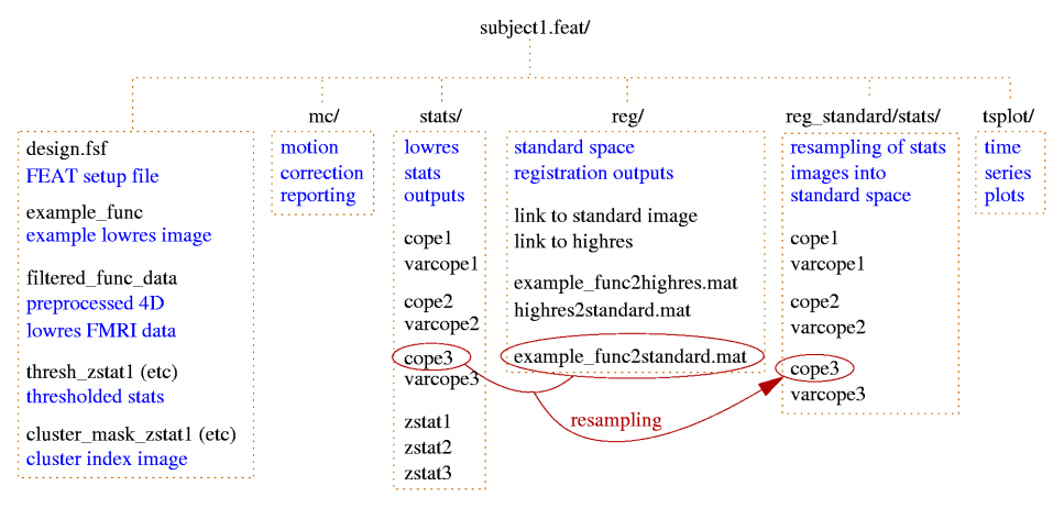
First-level FEAT output

File name	Description
cluster_mask_zstat1	image of clusters found for contrast 1; the values in the clusters are the index numbers as used in the cluster list.}
cluster_zstat1.html / .txt	the list of significant clusters for contrast 1. Note that the co-ordinates are the original voxel co-ordinates.
cluster_zstat1_std.html / .txt	the same, but with co-ordinates given in standard space. This exists if registration to standard space has been carried out.
design.con	list of contrasts requested.
design.fsf	FEAT setup file, describing everything about the FEAT setup. This can be loaded into the FEAT GUI.
design.fts	list of F-tests requested.
design.gif	2D image of the design matrix.
design.mat	the actual values in the design matrix.
design.trg	event onset times, created to be used in peri-stimulus timing plots.
design_cov.gif	2D image of the covariance matrix of the design matrix.
example_func	the example functional image used for colour rendering, and also the one that was used as the target in motion correction. This is saved before any processing is carried out. This is also the image that is used in registration to structural and/or standard images.
filtered_func_data	the 4D FMRI data after all filtering has been carried out. (prefiltered_func_data is the output from motion correction and the input to filtering, and will not normally be saved in the FEAT directory.) Although filtered_func_data will normally have been temporally high-pass filtered, it is not zero mean; the mean value for each voxel's timecourse has been added back in for various practical reasons. When FILM begins the linear modelling, it starts by removing this mean.
lmax_zstat1.txt / _std.txt	are lists of local maxima within clusters found when thresholding.
mask	the binary brain mask used at various stages in the analysis.
rendered_thresh_zstat1.png	2D colour rendered stats overlay picture for contrast 1.
rendered_thresh_zstat1	3D colour rendered stats overlay image for contrast 1. After reloading this image, use the Statistics Colour Rendering GUI to reload the colour look-up-table.
report.log	a log of all the programs that the feat script ran (ie the same as report.log but without the log outputs).
report.html	the web page FEAT report (see below).
thresh_zstat1	the thresholded Z statistic image for contrast 1.
mc/prefiltered_func_data_mcf.par	a text file containing the rotation and translation motion parameters estimated by MCFLIRT, with one row per volume.
mc/mc_rot.gif /_trans.gif	plots showing these parameters as a function of volume number (i.e., time).
reg/example_func2highres.*	files are related to the registration of the low res FMRI data to the high res image. The .mat file is the transformation in raw text format. The .gif image includes several slices showing overlays of the two images combined after registration. (Note that the inverse of each transform file is also saved (e.g. highres2example_func.mat) to make it easy for you later to take the highres image back into the lowres space.)
reg/example_func2standard.*	files are related to the registration of the low res FMRI data to the standard image.
reg/highres	a copy of the high res image.
reg/highres2standard.*	files are related to the registration of the high res image to the standard image.
reg/standard	is a symbolic link to the standard image.
stats/contrastlogfile	a logfile showing how well the statistics fit a Gaussian distribution, on the assumption of no activation.
stats/cope1	the contrast of parameter estimates image for contrast 1.
stats/corrections	the normalised covariance of the EV estimates; there is one volume for each element of the nEV x nEV covariance; it is normalised in that the actual covariance requires scaling by the residual variance, sigmasquares.
stats/dof	the mean estimated degrees-of-freedom over the whole data set.
stats/neff1	a statistical correction image for contrast 1.
stats/glslogfile	a FILM run logfile.
stats/pe1	the parameter estimate image for EV 1.
stats/probs	a list of probabilities used for estimating Gaussian statistical fitting.
stats/ratios	a list of estimates for Gaussian statistical fitting.
stats/sigmasquareds	the 3D image of the residual variance from the linear model fitting.
stats/smoothness	the estimation of the smoothness of the 4D residuals field, used in inference.
stats/stats.txt	another FILM logfile.
stats/threshac1	The FILM autocorrelation parameters.
stats/tstat1	the T statistic image for contrast 1 (\(=cope/\sqrt{varcope}\)).
stats/varcope1	the variance (error) image for contrast 1.
stats/zstat1	the Z statistic image for contrast 1
tsplot/tsplot_zstat1.gif	the full model vs data plot for the maximum Z statistic voxel from contrast 1.
tsplot/tsplot_zstat1p.gif	the plot of reduced data vs cope partial model fit - i.e. data-full_model+partial_model vs partial_model.
tsplot/tsplot_zstat1.txt	text file of values used for the above plots, for the maximum Z statistic voxel from contrast 1. The first column is the data, the second column is the partial model fit for contrast 1, the third column is the full model fit and the fourth column is the reduced data for contrast 1.
tsplot/tsplotc_zstat1.*	plots and text file as above, but instead of using the peak Z stat voxel, here the data is averaged over all voxels in all significant clusters for contrast 1.
ps_tsplot_zstat1_ev1.gif (etc)	peristimulus text files and plots, showing model fits averaged over multiple stimulus repeats and "data scatter" over these repeats. The format for the text files is the same as above, except for the insertion of an extra first column which encodes the peristimulus timing (i.e., time relative to the start time within the peristimulus window). The _ev1 part of the filename means that this file/plot relates to EV1; separate plots and text files are generated for each EV for every contrast.

If you have run F-tests as well as T-tests then there will also be many other files produced by FEAT, with filenames similar to those above, but with zfstat appearing in the filename.

The web page report includes the motion correction plots, the 2D colour rendered stats overlay picture for each contrast, the data vs model plots, registration overlay results and a description of the analysis carried out.

Time-series plots

FEAT generates a set of time-series plots for data vs model for peak Z voxels. The main FEAT report web page contains a single plot for each contrast (from the peak voxel); clicking on this takes you to more plots related to that contrast, including also, in the case of cluster-based thresholding, plots averaged over all significant voxels.

Plots of full model fit vs data show the original data and the complete model fit given by the GLM analysis.

Plots of cope partial model fit vs reduced data show the model fit due simply to the contrast of interest versus that part of the data which is relevant to the reduced model (i.e. full data minus full model plus cope partial model). This generally is only easily interpretable in the case of simple non-differential contrasts.

Peri-stimulus plots show the same plots as described above but averaged over all "repeats" of events, whether ON-OFF blocks in a block-design, or events in an event-related design. Thus you get to see the average response shape. Note that FEAT tries to guess what an "event" is in your design automatically, so in complex designs this can give somewhat strange looking plots! The peri-stimulus plots are for the peak voxel only; one pair of full/partial plots is produced for each EV in the design matrix for that peak voxel, with the "events" defined from that EV only.

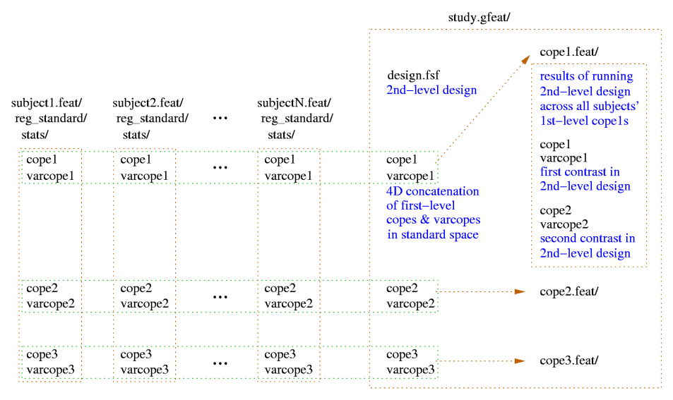
Higher-Level FEAT Output

A second-level .gfeat directory contains one 4D cope* for each of the first-level contrasts; these are simply the concatenation (across the first-level analyses) of those first-level cope images (in standard space) - ie the 4th dimension here is the number of first-level analyses. This is the input to the second-level analysis.

After the second-level analysis has completed each of those 4D cope* files in the .gfeat directory will have resulted in a .feat second-level output, containing all analysis steps (and of course, second-level output copes).

Additional files created include:

File name	Description
cope1.feat/filtered_func_data	the 4D file that collects the COPEs from the first level analyses, for contrast 1.
cope1.feat/var_filtered_func_data	the 4D file that collects the VARCOPEs from the first level analyses, for contrast 1.
cope1.feat/stats/mean_random_effects_var1	the estimate of the pure between-subjects random effect variance, for contrast 1.
cope1.feat/stats/weights1	4D file that is the reciprocal of the sum of of the 1st level VARCOPES and pure between-subjects random effect variance; the square root of this file are the weights used to whiten data and model as part of Generalised Least Squares, for contrast 1.