FLOBS

HRF basis functions

FLOBS (FMRIB's Linear Optimal Basis Sets) is a toolkit based around the idea of generating optimal basis sets for use in HRF convolution in FMRI linear modelling such as in FEAT. It allows the specification of sensible ranges for various HRF-controlling parameters (delays and heights for the different parts of the HRF "curve"), generates lots of example HRFs where each timing/height parameter is randomly sampled from the range specified, and then uses PCA to generate an optimal basis set that maximally "spans the space" of the generated samples.

It is easy to tell FEAT to use a FLOBS-generated basis set; either use the Make_flobs GUI or use the default FLOBS basis set supplied with FSL. Just select the optimal/custom HRF convolution option in the FEAT model setup.

It is also possible to use filmbabe instead of the normal FEAT timeseries analysis (which uses the FILM program). The difference is that filmbabe re-projects the optimal basis set onto the original complete set of samples so that it can learn priors on the expected means and covariances of the individual basis functions. This is so that these priors can then be used when fitting the model to the data, which means that the basis set is restricted from creating implausible HRF shapes. This means that the noise is less "randomly fit" by the model, giving better separation between the null part of the final statistics map and the activation part, i.e. better activation modelling power. Beware: note that the filmbabe program itself is relatively untested.

For more detail on FLOBS see:

M.W. Woolrich, T.E.J. Behrens, and S.M. Smith. Constrained linear basis sets for HRF modelling using Variational Bayes. NeuroImage, 21:4(1748-1761) 2004 and a related technical report TR04MW2.

`Make_flobs`

HRF basis functions

You can create your own optimal basis set using the Make_flobs GUI; either type Make_flobs from the command line, or find it under the Utils button in the FEAT GUI. The GUI is fairly self-explanatory; using the figure that appears, showing the HRF and its different controlling parameters (time widths set in seconds and the height parameter relative to the main peak height, which is set at 1), set the range you wish for each parameter. Press Preview and the basis set will be generated (with a reduced number of samples for speed), popping up a web browser window with the results, typically in a minute or less. The eigenvalues plot shows the eigenvalues for the most important basis functions which explain 99.5% of the variance. This might help you to refine your choice of the number of basis functions to use.

Now select an output directory name for the basis function information to get saved into (e.g. /Users/karl/my_basis_set.flobs) and press Go. Now the full number of samples will be generated and all necessary data (primarily the basis functions and their means and covariances when re-projected back onto the samples) will get saved for use in FEAT or in filmbabe.

If you are using the basis set inside FEAT, just select the optimal/custom HRF convolution option in the FEAT model setup GUI (for ALL relevant EVs!) and use the adjacent file browser button to change the default FLOBS directory to the one you have just created (again, you must do this for ALL relevant EVs).

`filmbabe`

If you want to try the filmbabe program (don't forget it hasn't been heavily tested) then you should do the following:

Read the paper or techrep linked to above.
Create your optimal basis set using Make_flobs.
Run FEAT as normal, using this new basis set.
Use filmbabescript as an easy way to run filmbabe, carry out inference (thresholding) and generate a web-page report. The usage is:
```
filmbabescript <feat_directory> <flobs_directory>
```

Note that the stats output from filmbabe does not follow a simple understood null-distribution (in the null case) so the standard methods for thresholding (like those currently used in FEAT) are not valid. Therefore filmbabescript makes use of the mm spatial mixture modelling program, which explicitly models both the null and the activation parts of the final stats image, allowing valid inference.

Group Level Analysis with Basis Functions

There are two main options open to you:

The typically taken approach is to only pass up to the group level the canonical HRF regression parameter estimates. This makes for a simple group analysis (with some variable sensitivity), and the benefits of including the basis function at the first level are still felt in terms of accounting for HRF variability, without which: - there would be increased error in the first level GLM fit - the explanatory power of certain first level original EVs may be overstated
Calculate a size summary statistic from the single session analyses (e.g., the amplitude at the peak of the HRF response - note that this is more interpretable than quantities like the zfstats, or the root mean square of the HRF basis function regression parameter estimates), and pass that up to the group level. However, the population distribution of such summary statistics will be non-Gaussian, and so non-parametric randomisation will be needed at the group level. Note that currently the amplitude at the peak of the HRF response is not provided by FEAT... so you would need to calculate that yourself.

There is a bit of extra detail needed to make option 2) work. This is because for main effects such size summary statistics will not be symmetrically distributed around zero under the null. This does not happen with differential (e.g. 1 -1) contrasts, as long as the contrasts are computed on the size summary statistics. For main effects, a way to overcome the problem would be to find the direction of the response for an original EV (e.g. by looking at the sign of the regression parameter for the main canonical HRF basis function regressor), and then to apply this sign to the size summary statistic.

For more details read on.

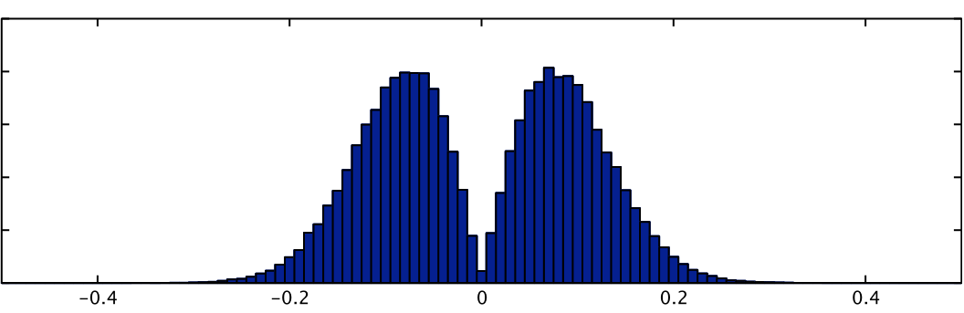
Summary statistics of a basis function fit can be calculated and passed up for higher-level analysis but only using non-parametric inference, such as randomise, due to the fact that the null distribution of these statistics is often highly non-Gaussian. For example, the signed RMS statistic (representing a form of "energy" of the linear combination, and as used in Calhoun et al, NeuroImage 2004) is:

sign(PE1)*sqrt(A1*PE12 + A2*PE22 + ...)

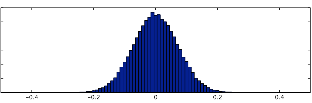
where PE1, PE2, etc are the parameter estimates associated EV1, EV2, etc., (all part of a basis function set for a single condition) and A1, A2, etc are weighting functions, typically equal to the mean square value of the respective EVs. The null distribution for this statistic is shown below, next to that of PE1 (where the latter is truly Gaussian). This highlights severity of the non-Gaussianity in such statistics.

RMS statistic	PE1

One exception to the use of non-parametric inference for such statistics is where there is a large number of subjects (or sessions) so that the Central Limit Theorem can be invoked. For highly non-Gaussian distributions this can require a significant number of subjects.

Once a scalar statistic has been calculated from each first level result, the collection of such images can be merged with fslmerge and then passed into randomise for non-parametric testing. Note that in order to avoid problems with non-differential contrasts (e.g. single group averages) the statistic should be made to be symmetric under the null hypothesis, such as was done with the sign(PE1) term above.

As there is no single statistic of universal interest there are no standard tools for calculating these at present. Users are recommended to use Matlab or similar tools to calculate their statistics of interest (which usually require the combination of information in the PE images and in the EV files, where the latter can be obtained from the design.mat within FEAT).