ProbtrackX - probabilistic tracking with crossing fibres
For details about probabilistic tractography as implemented in FDT, see this technical report, and for details about crossing fibre modelling in FDT, see Behrens et al, NeuroImage 2007.
After bedpostx has been applied it is possible to run tractography analyses using probtrackx. Briefly, probtrackx produces sample streamlines, by starting from some seed and then iterates between (1) drawing an orientation from the voxel-wise bedpostX distributions, (2) taking a step in this direction, and (3) checking for any termination criteria. These sample streamlines can then be used to build up a histogram of how many streamlines visited each voxel or the number of streamlines connecting specific brain regions. This streamline distribution can be thought of as the posterior distribution on the streamline location or the connectivity distribution.
The remainder of this page is organied into the following sections:
Running ProbtrackX
The following explains how to run probtrackx. The GUI can be started using Fdt (fdt_gui on the mac). The command-line options (which are more flexible than the GUI) can be viewed using:
Note that the GUI only runs the new version (probtrackx2). Users of the old version (probtrackx) can only run it from the command line.
PROBTRACKX requires the specification of a bedpostX directory. This directory must contain all the following images:
-
merged_th<i>samples.nii.gz -
merged_ph<i>samples.nii.gz -
merged_f<i>samples.nii.gz -
nodif_brain_mask.nii.gz
Here we will first discuss how to use seed, termination, waypoint, and exclusion masks to select a specific subset of all possible streamlines (i.e., to guide the tractography). Afterwards, we will present the various probtrackx outputs. Finally, we have a section on using surface masks in probtrackx.
Guiding the tractography
A whole range of tools is available to guide the tractography. The most powerful of these is to select the seed region, which defines where the streamlines originate. In addition to this we can set termination masks to stop the streamlines, and waypoint/exclusion masks to filter out those streamlines not relevant for our analysis (e.g., filter out the streamlines not part of our white matter tract of interest).
Info
Every target mask must be in the same space as the seed masks (or the reference image in the case of a single voxel or surface seed). Any surface must also use the same convention (i.e. FreeSurfer/Caret/FIRST/voxel - see below).
The results from probtrackx will be binned in the same space as the input masks. More information on selecting this space is provided below.
Seed specification
The seed can be specified in three different ways (selected in the GUI in the Data tab):
-
Single voxel seed: Generates streamlines from a single user-specified voxel. In the GUI this voxel is defined by setting the x,y,z coordinates in voxels or millimetres. From the command line this is enabled by providing a text file with the voxel coordinates to the
-x,--seedflag and setting the--simpleflag. -
Single mask: This is the most common setting, where the seed region is defined by a user-provided mask. Streamlines are seeded from each voxel in the mask. This mask can either be a volumetric (i.e., NIFTI) file or a surface file. On the command line this is achieved by passing on a NIFTI or surface filename to the
-x,--seedflag. -
Multiple masks: Streamlines are seeded from each of the masks. This can be used to generate streamlines from both a volumetric and surface mask or to produce an ROIxROI connectivity matrix. All the masks have to be in the same space and surface masks need to use the same encoding.
If the seed is a single voxel or a surface, a reference image will also need to be provided (--seedref on the command line).
The number of individual streamlines (or samples) that are drawn in each voxel or surface vertex can be set using the -P/--nsamples flag or in the Options>Basic Options section in the GUI. By default this is set to 5000 as we are confident that convergence is reached with this number of samples. However, reducing this number will speed up processing and can be useful for preliminary or exploratory analyses.
By default, each streamline will be initialised in the centre of each voxel (or at the surface vertex location). This can be changed to sample in a sphere around the voxel centre or vertex using the --sampvox flag or in the Options>Advanced Options section in the GUI.
Waypoint masks
If set, only streamlines that pass through the waypoint mask will be considered valid. Invalid streamlines are not counted when producing the various probtrackx outputs. These can be set in the GUI Data tab or using the --waypoints flag.
If more than one mask is set, then by default probtrackx will perform an AND operation. I.e. tracts that do not pass through ALL these masks will be discarded from the calculation of the connectivity distribution. You can set this to an OR using the Options>Waypoint option section in the GUI (--waycond on the command line). In this case, streamlines are retained if they intersect at least one of the waypoint masks. In the GUI use the add and remove buttons to make a list of waypoint masks. On the command line provide an ASCII file with the list of waypoint masks to the --waypoints flag.
Waypoint masks can be made more strict by selecting Force waypoint crossing in selected order in the Options>Waypoint option section in the GUI (--wayorder on the command line). With this option only streamlines are accepted that cross the waypoint mask in the order provided in the GUI or text file. Any streamline that reaches a waypoint out of order is terminated and rejected. This is only used when the waypoint condition is set to AND.
Exclusion mask
If an exclusion mask is to be used then check the box in the Data tab of the GUI and use the browse button to locate the mask file (or use the --avoid flag on the command line). Pathways will be discarded if they enter the exclusion mask. For example, an exclusion mask of the midline will remove pathways that cross into the other hemisphere.
Termination mask
If a termination mask is to be used then check the box and use the browse button to locate the mask file (or use the --stop flag on the command line). Pathways will be terminated as soon as they enter the termination mask. The difference between an exclusion and a termination mask is that in the latter case, the tract is stopped at the target mask, but included in the calculation of the connectivity distribution, while in the former case, the tract is completely discarded. (Note that paths are always terminated when they reach the brain surface as defined by nodif_brain_mask)
Streamlines are terminated as soon as they reach this mask. If you want to only terminate the streamlines once they leave the provided mask use the --wtstop mask instead. This can be useful to track streamlines through some termination mask without allowing them to leave. Streamlines that are seeded within the --wtstop mask are allowed to leave once without being terminated immediately.
Termination/exclusion criteria
Streamlines are terminated, when one of the following criteria is fulfilled:
- A termination or exclusion mask is used (see above).
-
The streamline leaves the
nodif_brain_maskin the input bedpostX directory. -
The maximum number of steps is reached. By default, samples are terminated when they have travelled 2000 steps. Using the default step length of 0.5mm this corresponds to a distance of 1m. Adjust using Options>Advanced Options GUI section or
-S,--nstepson the command line. -
The curvature of the next step is too high compared with the previous one. We limit how sharply pathways can turn in order to exclude implausible pathways. This number is the cosine of the minimum allowable angle between two steps. By default this is set to 0.2 (corresponding to a minimum angle of approximately ±80 degrees). Adjusting this number can enable pathways with sharper angles to be detected (Options>Basic Options GUI section or
-c,--cthron the command line). -
The streamline loops back on itself -i.e paths that travel to a point where they have already been. In the GUI this is enabled by default (see Options>Basic Options). It can be activated on the command line using
-l,--loopcheck. -
The fractional anisotropic volumes (stored in
merged_f<i>samples.nii.gz) can be used to influence the tractography. If activated (Options>Advanced Options in the GUI;-f,--usefon the command line) the tracts stop if the anisotropy is lower than a random variable between 0 (low anisotropy) and 1 (high anisotropy).
When terminated, the next step is to determine whether the streamline is valid (i.e., whether it will be counted in the probtrackx output). Streamlines are invalid if one of the following is true:
- The streamline reached the exclusion mask.
- The waypoint constraints were not met (see above for the various options)
- The total streamline length is shorter than some user-defined threshold. This minimum threshold is disabled by default (i.e., all streamlines pass this test). It can be set in the Options>Advanced Options GUI section or using the
--disttrhreshflag on the command line. - None of the target regions were reached when using the
--networkflag to compute an ROIxROI connectivity matrix (see below).
Masks in non-diffusion space
All masks must be provided in the same space (i.e., the NIFTI files must have the same size and be registered with each other). The output files will be produced in this same space. By default, probtrackx will assume that this space is diffusion space, however the masks can also be provided in a different space by selecting Seed space is not Diffusion on the GUI Data tab or using the --xfm and/or --invxfm.
If the transformation to the diffusion space is linear (e.g., for masks from a subject-specific structural image) only the transformation matrix from seed space to diffusion space has to be provided (using the --xfm flag on the command line). For non-linear transforms (e.g., for masks in standard space) the FNIRT non-linear transform has be provided both from seed space to diffusion space (--xfm) and from diffusion space to seed space (--invxfm).
For example, for analyses in structural space:
-
Linear:
xfms/str2diff.mat -
Nonlinear:
xfms/str2diff_warpandxfms/diff2str_warp
The actual registration step to get these affine and non-linear transforms is discussed the registration section.
Adjust streamlines path
Here we list some options available to adjust the path streamlines take (as opposed to controlling seeding, terminating, and rejecting them). These are available in the Advanced Options section in the Options tab of the GUI or with the command line flags listed:
-
Modified Euler streamlining (
--modeuler): Use modified Euler integration as opposed to simple Euler for computing probabilistic streamlines. More accurate but slower. -
Step length (
-S,--nsteps; default 0.5mm): This determines the length of each step. This setting may be adjusted from default e.g., depending on the voxel size being used, or if tracking is being performed on different sized brains (e.g., infants or animals). -
Subsidiary fibre volume threshold (
--fibthresh; default=0.01): Threshold on the volume fraction of subsidiary fibres. Fibres with a lower volume fraction than this threshold (as given in themean_f<i>samples.nii.gzfile in thebedpostxdirectory) are discarded during tractography.
Probtrackx outputs
The seed, termination, waypoint, and exclusion masks defined above determine which streamlines will be counted in the probtrackx output files. Here we will discuss the various output files available.
A successful run of probtrackx will produce the following files in the output directory:
-
probtrackx.log- a text record of the command that was run. This file can be useful to rerun the same or a slightly altered version ofprobtrackx. -
fdt.log- a log of the setup of the FDT GUI when the analysis was run. To recover this GUI setup, typeFdt fdt.log. This file is only produced if run from the GUI. -
waytotal- a text file containing a single number corresponding to the total number of generated tracts that have not been rejected by inclusion/exclusion mask criteria.
All probtrackx outputs count the number of streamlines in some way. The option Use distance correction (Options>Advanced Options in GUI or --pd flag) corrects for the fact that connectivity distribution (i.e., number of streamlines) drops with distance from the seed mask. If this option is checked, the connectivity distribution is the expected length of the pathways that cross each voxel times the number of samples that cross it.
In addition to counting the number of streamlines, the average length of the streamlines up to that point can also be stored by setting the --ompl flag in addition to setting at least one of the output listed below.
Streamline density map
This is the default output when running from the GUI (activate using the --opd flag in the probtrackx output). The result is a 3D image file (called fdt_paths.nii.gz) containing the number of streamlines reaching each voxel. This can be thought of as quantifying the connectivity from the seed region.
By carefully selecting the seed region, termination mask, and inclusion/exclusions masks, this can be used to reconstruct specific white matter tracts. For example, XTRACT leverages probtrackx and a set of carefully curated masks to reconstruct many of the major white matter tracts.
ROI by ROI connectivity matrix
The output here quantifies the number of streamlines seeded in one region of interest (ROI) that reached another ROI. For N ROIs, the result will be an NxN matrix (called fdt_network_matrix), where each row quantifies how many streamlines seeded in a certain ROI reached the other ROIs.
In the GUI this output can be produced by providing the N ROIs as multiple seed masks (see above for instructions). An ASCII text file listing the ROIs can also be provided on the command line. On the command line the --network flag should also be added to produce the NxN matrix.
Voxel by ROI connectivity
To estimate the voxelxROI connectivity probtrackx quantifies connectivity values between each voxel in a seed mask and any number of user-specified target masks. In the example above, seed voxels in the thalamus are classified according to the probability of connection to different cortical target masks.
In the GUI this output is created by selecting Classification Targets on the Data tab (note that this option is only available if the seed space is set to Single Mask). Use the add button to locate each target mask. Targets must be in the same space as the seed mask. When all targets are loaded you can press the save list button to save the list of targets as a text file. If you already have a text file list of required targets (including their path) then you can load it with the load list button or set the --targetmasks and --os2t flags on the command line.
The output directory will contain a single volume for each target mask, named seeds_to_{target}.nii.gz where {target} is replaced by the file name of the relevant target mask. In these output images, the value of each voxel within the seed mask is the number of samples seeded from that voxel reaching the relevant target mask. The value of all voxels outside the seed mask will be zero. Note that the files seeds_to_{target}.nii.gz will have the same format (either volumes or surfaces) as the seed mask.
There are command line utilities that can be run on these outputs:
proj_thresh- for thresholding some outputs ofprobtrackxfind_the_bigggest- for performing hard segmentation on the outputs ofprobtrackx, see example below
Voxel by voxel connectivity matrix
Voxel by voxel connectivity matrices are available in the GUI through the Matrix Options in the Options tab or using --matrix1/2/3 and associated flags in the command line (see probtrackx2 --help).
These can be used to store a connectivity matrix between 1. all seed points and all other seed points, or 2. all seed points and all points in a target mask, or 3. all pairs of points in a target mask (or a pair of target masks).
These options can be used separately or in conjunction.
Info
All masks used here MUST BE IN SEED SPACE.
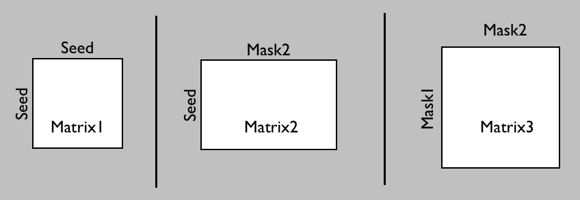
Matrix1 and Matrix2 store the number of samples (potentially modulated by distance when distance correction is used) between the rows (seed points) and the columns of the matrix.
Matrix3 stores the number of sample streamlines (potentially modulated by distance when distance correction is used) between each pair of points in a pair of target masks. In this case, when a streamline is sent from each seed point in both directions, if the streamline hits the two target masks at two locations along either sides of the streamline, the corresponding row and column of matrix3 is filled.
Note on the output format: matrix1,2,3 are stored as 3 column ASCII coding of sparse matrices. These files can be loaded into matlab using e.g.:
or in Python using:
import scipy.sparse as sps
import numpy as np

# Helper function for loading matlab-style sparse matrix
def load_spmat(matfile):
    spmat   = np.loadtxt(matfile)
    v, r, c = mat[:-1, -1], np.array(mat[:-1, 0]-1, dtype=int), np.array(mat[:-1, 1]-1, dtype=int)
    nr, nc  = int(mat[-1, 0]), int(mat[-1,1])
    return sps.csc_matrix((v, (r, c)), shape=(nr, nc)).toarray()

# load the matrix file into a numpy array
M = np.loadtxt('fdt_matrix1.dot')
Typical uses of Matrix options:
- Matrix1: The seed mask(s) can represent grey matter, so this would be all GM to GM connectivity.
- Matrix2: The seed can be a grey matter region, and mask2 the rest of the brain (can be low res). The results can then be used for blind classification of the seed mask.
- Matrix3: The 'target' masks can be the whole of grey matter, and the seed mask white matter. This option allows more sensitive reconstruction of grey-to-grey connectivity as pathways are seeded from all their constituting locations, rather than just their end-points as in Matrix1.
Example use of Matrix2 for clustering:
A typical use of Matrix2 is blind (i.e. hypothesis-free) classification. Say you have run probtrackx with a seed roi (e.g. thalamus) and the --omatrix2 option by setting the Matrix2 target mask to a whole brain mask (typically this mask would be lower resolution than the seed mask). The resulting Matrix2 can be used in Matlab to perform 'kmeans' classification. Below is an example Matlab code to do this (this example is only valid if the seed mask is a NIFTI volume, not a surface):
% Load Matrix2
x=load('fdt_matrix2.dot');
M=full(spconvert(x));
% Calculate cross-correlation
CC  = 1+corrcoef(M');
% Do kmeans with k clusters
idx = kmeans(CC,k);   % k is the number of clusters
% Load coordinate information to save results
addpath([getenv('FSLDIR') '/etc/matlab']);
[mask,~,scales] = read_avw('fdt_paths');
mask = 0*mask;
coord = load('coords_for_fdt_matrix2')+1;
ind   = sub2ind(size(mask),coord(:,1),coord(:,2),coord(:,3));
[~,~,j] = unique(idx);
mask(ind) = j;
save_avw(mask,'clusters','i',scales);
!fslcpgeom fdt_paths clusters
And below is an equivalent code using Python and fslpy:
# Load Matrix2
M = load_spmat(matfile)
# Calculate cross-correlation
CC  = 1+np.corrcoef(M)
# Do kmeans with k clusters
from sklearn.cluster import KMeans
idx = KMeans(n_clusters=2).fit_predict(CC)   # k is the number of clusters
# Load coordinate information to save results
from fsl.data.image import Image
img = Image('fdt_paths.nii.gz')
mask = 0*img.data;
coord = np.loadtxt('coords_for_fdt_matrix2', dtype=int);
# Create image with clustering and save results
ind   = np.ravel_multi_index((coord[:,0],coord[:,1],coord[:,2]), img.shape)
mask[ind] = idx
out = Image(mask, header=img.header)
out.save("clusters.nii.gz")
Using surfaces
It is possible to use surface files in probtrackx. The preferred format is GIFTI.
Surface files typically describe vertex coordinates in mm. Annoyingly, different softwares use different conventions to transform mm to voxel coordinates. Probtrackx can deal with the following conventions: freesurfer, caret, first and voxel. The latter convention simply means that mm and voxel coordinates are the same.
Switching conventions
When using surfaces in probtrackx, all surfaces MUST use the same convention. However, we provide a command-line tool (surf2surf) to transform between different conventions. This tool can also be used to convert between different surface file formats.
surf2surf -i <inputSurface> -o <outputSurface> [options]

Compulsory arguments (You MUST set one or more of):
        -i,--surfin     input surface
        -o,--surfout    output surface

Optional arguments (You may optionally specify one or more of):
        --convin        input convention [default=caret] - only used if output convention is different
        --convout       output convention [default=same as input]
        --volin         input ref volume - Must set this if changing conventions
        --volout        output ref volume [default=same as input]
        --xfm           in-to-out ascii matrix or out-to-in warpfield [default=identity]
        --outputtype    output type: ASCII, VTK, GIFTI_ASCII, GIFTI_BIN, GIFTI_BIN_GZ (default)
        --values        set output scalar values (e.g. --values=mysurface.func.gii or --values=1)
Projecting data onto the surface
It is often useful to project 3D data onto the cortical surface. We provide the following command-line tool (surf_proj) to do exactly that:
Usage: surf_proj [options]

Compulsory arguments (You MUST set one or more of):
        --data  data to project onto surface
        --surf  surface file
        --out   output file

Optional arguments (You may optionally specify one or more of):
        --meshref       surface volume ref (default=same as data)
        --xfm   data2surf transform (default=Identity)
        --meshspace     meshspace (default='caret')
        --step  average over step (mm - default=1)
        --direction     if>0 goes towards brain (default=0 ie both directions)
        --operation     what to do with values: 'mean' (default), 'max', 'median', 'last'
        --surfout       output surface file, not ascii matrix (valid only for scalars)
Using FreeSurfer surfaces
In order to use FreeSurfer-generated surfaces as masks in probtrackx, you need to add the following command line options (which can also be set in the GUI):
Where the orig.nii.gz file can be generated by converting the orig.mgz file (found in the FreeSurfer output directories) using FreeSurfer's mri_convert.
Additionally, using FreeSurfer with probtrackx requires a few specific steps that we describe below.
FreeSurfer Registration
FreeSurfer operates in a conformed space, which is different from the original structural image space that it has received as an input. When tracking from FreeSurfer surfaces, it is necessary to provide a transformation between conformed space and diffusion space. Below are a few steps that show how to achieve this.
We assume that you have ran dtifit on your diffusion data with an FA map called dti_FA.nii.gz (we recommend using an FA map to register to T1 structural images), and also that you have a file called struct.nii.gz that you have used as an input to FreeSurfer recon_all program.
We will carry on a few steps that aim at calculating the following transformations: fa<->struct<->freesurfer. Then we will concatenate these transformations to get fa<->freesurfer.
Let us start with struct<->freesufer (assuming john is the subject's name):
tkregister2 --mov $SUBJECTS_DIR/john/mri/orig.mgz --targ $SUBJECTS_DIR/john/mri/rawavg.mgz --regheader --reg junk --fslregout freesurfer2struct.mat --noedit
convert_xfm -omat struct2freesurfer.mat -inverse freesurfer2struct.mat
Now transforming FA to struct:
flirt -in dti_FA -ref struct_brain -omat fa2struct.mat
convert_xfm -omat struct2fa.mat -inverse fa2struct.mat
The final stage is to concatenate these transformations:
convert_xfm -omat fa2freesurfer.mat -concat struct2freesurfer.mat fa2struct.mat
convert_xfm -omat freesurfer2fa.mat -inverse fa2freesurfer.mat
Label files
Label files from FreeSurfer are useful as cortical ROIs for tractography. In order to use a label file (or collection of labels) in probtrackx, you must first transform it (them) into a surface file, using the label2surf command.
For instance, say you want to create a surface ROI for Brodmann areas 44 and 45. You must first decide which surface to use (pial, white) and which hemisphere (lh or rh). Say you want BA44/45 on the lh.white surface, then you must first transform the relevant surface file into an FSL-compatible format (ASCII or VTK or GIFTI), then use label2surf to transform the label files into a surface file. Below, the first command is a FreeSurfer command:
mris_convert lh.white lh.white.gii
echo lh.BA44.label lh.BA45.label > listOfAreas.txt
label2surf -s lh.white.gii -o lh.BA44.gii -l listOfAreas.txt
The full set of arguments for label2surf is shown below:
label2surf
         Transforms a group of labels into a surface

Usage:
label2surf -s <surface> -o <outputsurface> -l <labels>

Compulsory arguments (You MUST set one or more of):
        -s,--surf       input surface
        -o,--out        output surface
        -l,--labels     ascii list of label files

Optional arguments (You may optionally specify one or more of):
        -v,--verbose    switch on diagnostic messages
        -h,--help       display this message