Postmortem MRI
The brain was scanned postmortem over three sessions with ~270 hours of scanning data collected in total. Data were acquired on a 7T small animal scanner (Agilent) with a 400 mT/m gradient coil and Birdcage receive/transmit RF coil.
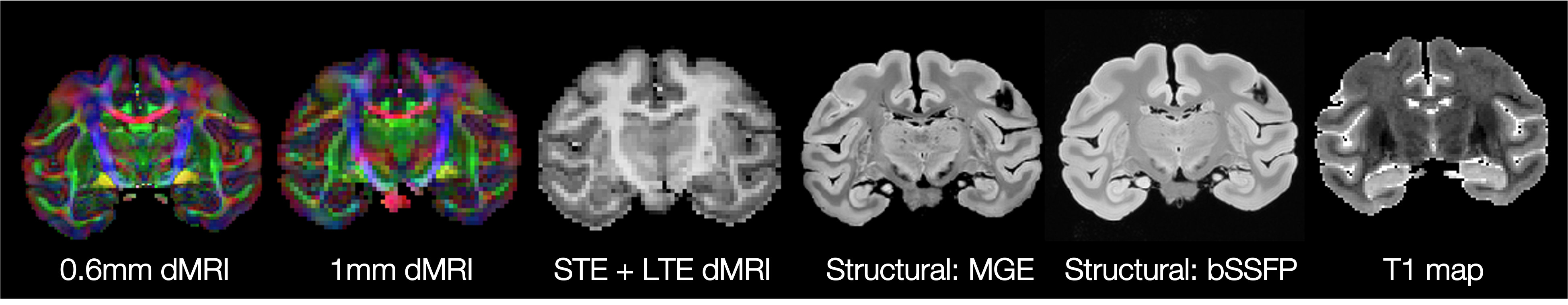
Below we summarise the postmortem MRI data acquired, and show example screen shots of preprocessed data to demonstrate its quality. The data includes diffusion MRI at 0.6mm and 1mm (incl. spherical tensor encoded dMRI at 1mm), two structural images at 0.3mm (MGE and bSSFP) and a T1 map at 0.6mm isotropic resolution.
The data were preprocessed using FSL tools. For further details see the NatComms paper and bigmacanalysis git repository (link via Code Availability).
Diffusion MRI
Diffusion MRI data were acquired with three main goals:
High spatial resolution (0.6mm)
Multi-shell, ultra-high angular resolution imaging (Ultra-HARDI) (1mm)
Multi-shell spherical tensor encoding (1mm)
All diffusion weighted images were acquired using a spin echo multi-slice (DW-SEMS) sequence and single-line readout to minimise image distortions.
High spatial resolution
High spatial resolution data were acquired at 0.6 mm isotropic resolution with a single shell and 128 gradient directions.
Acquisition parameters: TE/TR = 25.4 ms/10 s; FOV=76.8x76.8 mm; δ/Δ = 7/13 ms; time per gradient direction = 21.3 mins; b = 4 ms/μm2; 0.6 mm isotropic resolution; G = 32 G/cm; 128 gradient directions followed by 8 non-diffusion weighted volumes.
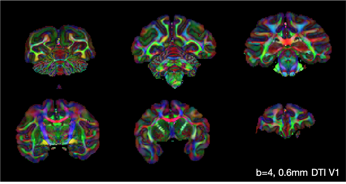
In the figure below, the diffusion tensor model was fitted to the b = 4 ms/μm2, 0.6 mm data. Here we show the primary eigenvector V1, weighted by the fractional anisotropy.
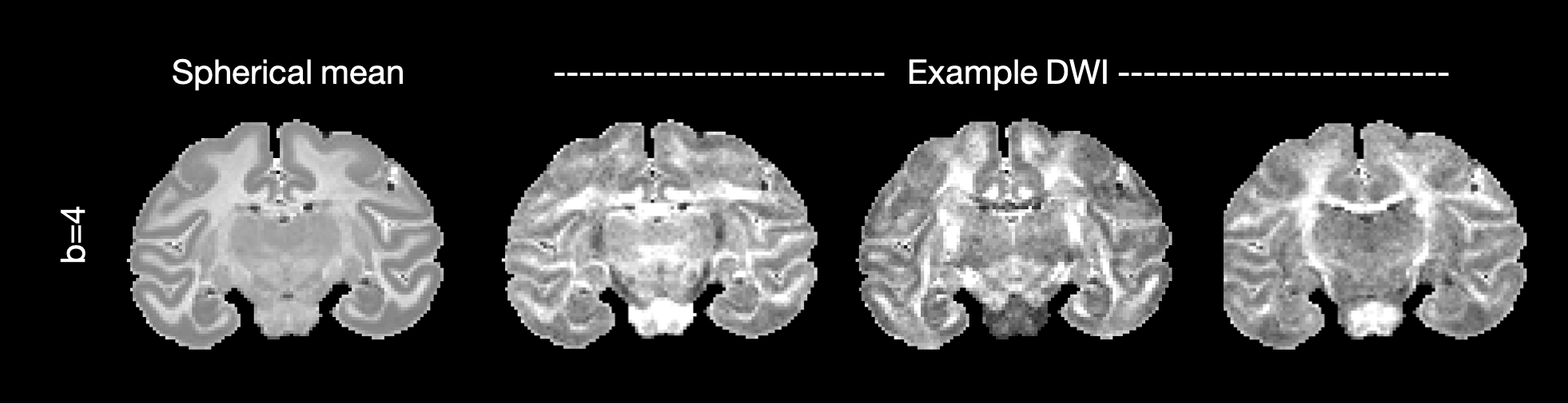
The figure below shows the average signal across DWI (spherical mean) and example DWI along three gradient directions.
Ultra-HARDI
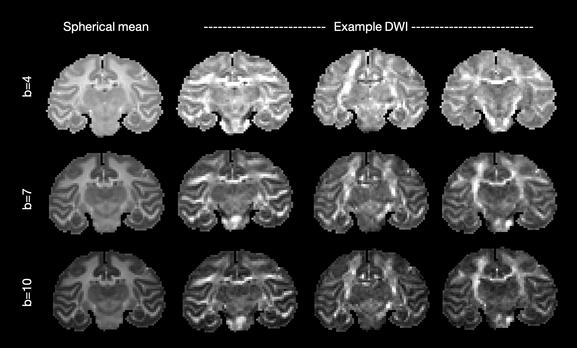
Multi-shell, ultra-HARDI data were acquired at 1 mm isotropic resolution with 250 gradient directions at b=4 ms/μm2 and 1000 gradient directions each at b=7,10 ms/μm2.
Acquisition parameters: TE/TR = 42.4 ms/3.5 s; FOV = 76 x 76 x 76 mm; δ/Δ = 14/24ms; 1 mm isotropic resolution; time per gradient direction = 4.1 mins; b=4 ms/μm2 data had G = 12.0 G/cm, 250 gradient directions and 10 non-diffusion weighted volumes; b=7 ms/μm2 had G = 15.9 G/cm, 1000 gradient directions and 40 non-diffusion weighted volumes; b = 10 ms/μm2 had G = 19.1 G/cm, 1000 gradient directions and 40 interspersed non-diffusion weighted volumes.
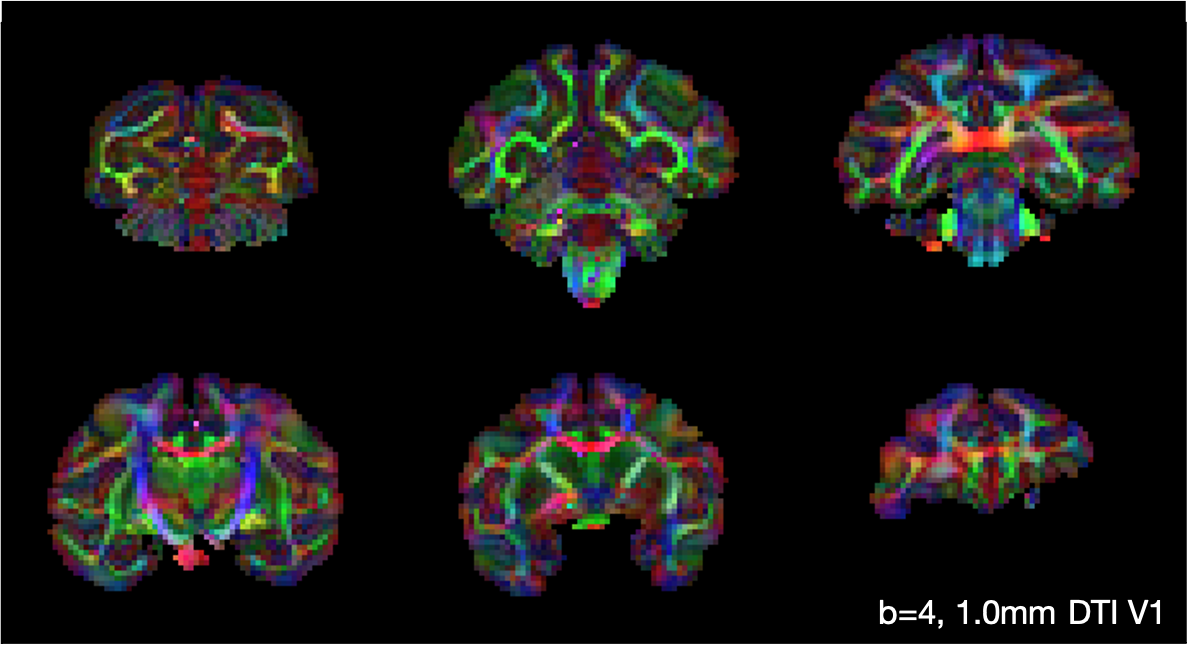
The figure below shows the primary eigenvector V1 of the diffusion tensor, weighted by the fractional anisotropy, when the diffusion tensor model (Basser1994) was fitted to the b = 4 ms/μm2, 1.0 mm data.
The figure below shows the average signal across DWI (spherical mean) and example DWI along three gradient directions for each b-value. Note the gradient directions for b = 4 ms/μm2 are not the exact same as those for b = 7,10 ms/μm2.
Spherical tensor encoding
Data combining linear and tensor encoding were acquired at 1 mm isotropic resolution with a slightly longer TR than the ultra-HARDI data. The gradient amplitude G was adjusted to produced the required b-values of b=4,7,10 ms/μm2.
Acquisition parameters for spherical encoding: TE/TR = 42.5 ms/6.4 s; FOV = 76 x 76 x 76 mm; 1 mm isotropic resolution. For each b-value, 30 images (averages) were acquired with spherical tensor encoding and 1 with negligible diffusion weighting.
Acquisition parameters for linear encoding: TE/TR = 42.5 ms/6.4 s; FOV = 76 x 76 x 76 mm; 1 mm isotropic resolution, δ/Δ = 14/24 ms, 50 gradient directions per shell plus 2 volumes with negligible diffusion weighting.
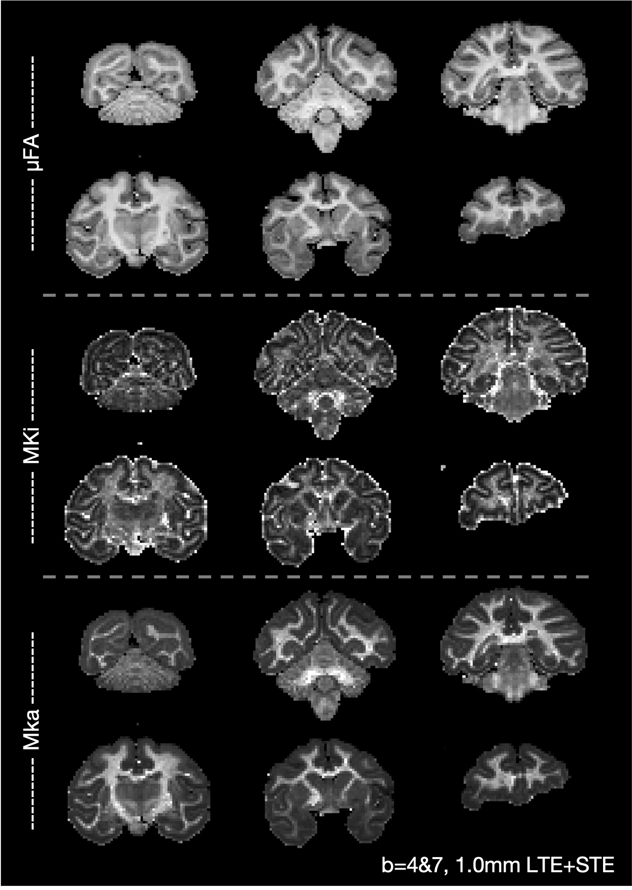
The figure below shows a map of the microscopic fractional anisotropy (μFA), isotropic microscopic kurtosis (MKi) and anisotropic microscopic kurtosis (MKa), where the Laplace transform of the gamma distribution (dtd_gamma model from the DIVIDE framework, Lasic2014,Szczepankiewicz2019,Nilsson2018) was fitted to the b = 4,7 ms/μm2, 1.0 mm data with linear and spherical encoding.
Structural MRI
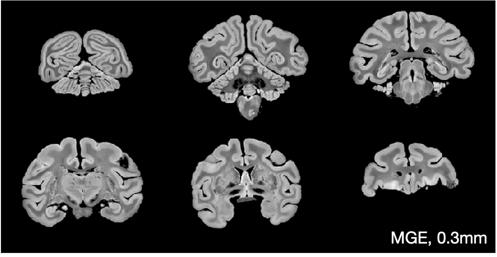
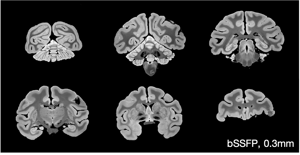
Two structural images were acquired at 0.3 mm isotropic resolution using 1) a multi-gradient echo sequence (MGE 3D) and 2) a balanced SSFP (bSSFP) sequence.
MGE acquisition parameters: TE/TR = 7.8/97.7 ms, flip angle 30 deg, 0.3 mm isotropic resolution, FOV = 76.8 x 76.8 x 76.8 mm.
bSSFP acquisition parameters: TRUFI sequence; 16 frequency increments; TE/TR = 3.05/6.1 ms, flip angle 30 deg, 0.3 mm isotropic resolution, FOV = 76.8 x 76.8 x 76.8 mm. Data was averaged using the root-mean sum of squares.
The figure below shows example MGE images which have been corrected for Gibbs ringing and bias field.
The figure below shows example bSSFP images which have been corrected for Gibbs ringing.
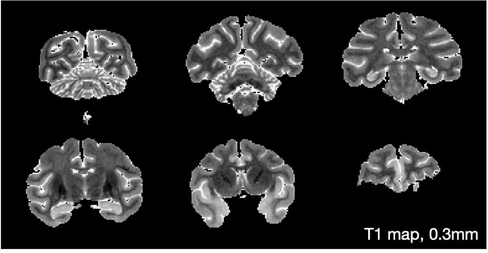
T1 mapping
A T1 map was generated from inversion recovery data at 0.6 mm isotropic resolution.
Acquisition parameters: TE/TR = 8.6 ms/10 s, 0.6 mm isotropic resolution, FOV = 76.8 x 76.8 x 76.8 mm and 12 inversion times (TI) from 10 to 6000 ms. Quantitative T1 maps were then fitted voxelwise using qMRLab (Karakuzu2020) and the Barral model (Barral2010): https://qmrlab.readthedocs.io/en/master/inversion_recovery_batch.html
A map of quantitative T1 is shown below.
Key references:
Basser, P.J., Mattiello, J., LeBihan, D.. MR diffusion tensor spectroscopy and imaging. Biophysical Journal 1994; 66(1):259-267. doi:10.1016/S0006-3495(94)80775-1.
Lasic S., Szczepankiewicz F., Eriksson S., Nilsson M., Topgaard D., Microanisotropy imaging: quanti cation of microscopic diffusion anisotropy and orientational order parameter by diffusion MRI with magic-angle spinning of the q-vector. Frontiers in Physics 2014;2:11. doi:10.3389/fphy.2014.00011.
Szczepankiewicz F., Lasic S., van Westen D., Sundgren P. C., Englund E., Westin C.-F., Stahlberg F., Latt J., Topgaard D., Nilsson M., Quantification of microscopic diffusion anisotropy disentangles effects of orientation dispersion from microstructure: Applications in healthy volunteers and in brain tumors. NeuroImage 2015;104:241{252. doi:10.1016/j.neuroimage.2014.09.057.
Nilsson M., Szczepankiewicz F., Lampinen B., Ahlgren A., de Almeida Martins J. P., Lasic S., Westin C., Topgaard D., An open-source framework for analysis of multidimensional diffusion MRI data implemented in MATLAB (2018), Proc. Intl. Soc. Mag. Reson. Med. 26, Paris, France
Karakuzu A., Boudreau M., Duval T., Boshkovski T., Leppert I. R., Cabana J.-F., Gagnon I., Beliveau P., Pike G. B., Cohen-Adad J., Stikov N., qMRLab: Quantitative MRI analysis, under one umbrella. Journal of Open Source Software 2020;5(53):2343. doi:10.21105/JOSS.02343.
Barral J. K., Gudmundson E., Stikov N., Etezadi-Amoli M., Stoica P., Nishimura D. G., A robust methodology for in vivo T1 mapping. Magnetic Resonance in Medicine 2010;64(4):1057{1067. doi:10.1002/MRM.22497.