Microscopy
After scanning, the brain was sectioned with consecutive slices allocated to one of six “sets” of sections processed for different microscopy contrasts. Five sets have sections that are 50 μm thick, one set of sections is 100 μm thick. There is a 350 μm gap between sections of the same contrast.
One set of sections were left unstained and mounted onto glass slides for polarised light imaging.
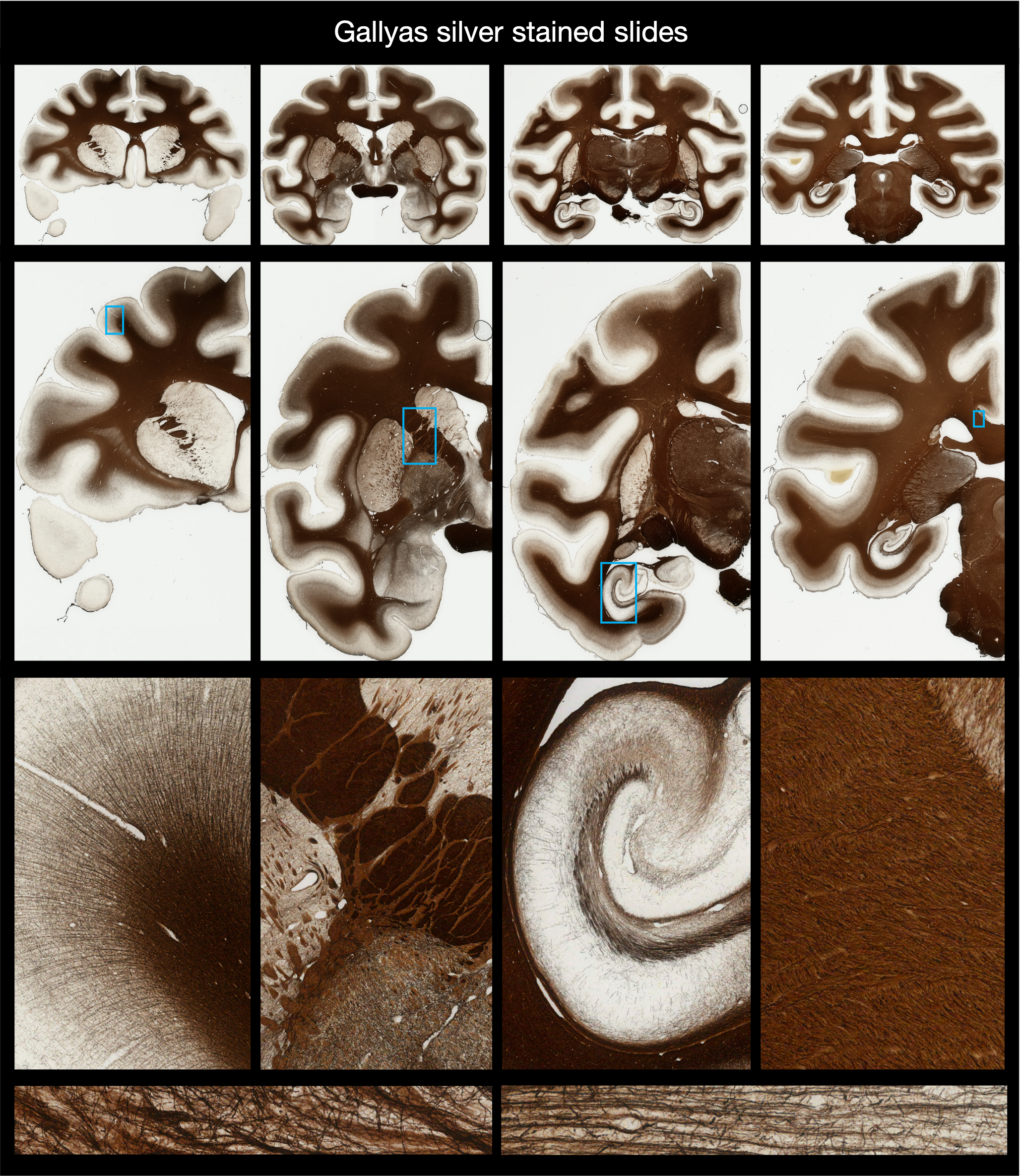
A second set was stained with Gallyas silver to visualise myelin.
A third set was stained with Cresyl violet to visualise Nissl bodies (data coming soon).
The final three sets of sections are currently unstained (2 sets 50 μm thick, 1 set 100 μm thick) and will be added in the future.
Further details on the microscopy data acquisition can be found in the paper.
Polarised light imaging
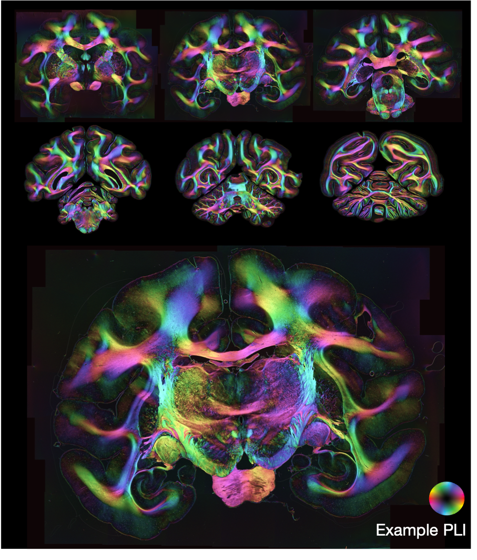
Polarised light imaging (PLI, Axer2011) utilises the birefringence of myelin to estimate the primary fibre orientation per microscopy pixel. The BigMac dataset includes 2D PLI at a resolution of ~ 4μm/pixel, where we infer maps of the transmittance, retardance and orientation of axons within the 2D microscopy plane (see definitions below).
PLI basics
Birefringence
Birefringence is an inherent optical property of certain materials that can act to alter the polarisation of incident light. When polarised light is incident on a birefringent material, it is split into two components according to the optic axis (the ordinary and extraordinary rays), where polarised light oriented along the optic travels at the different speed to that orthogonal to the optic axis. This creates a phase difference between the two ray components. Linear polarisation describes when the two rays are perfectly in phase, circular polarisation describes when the phase difference is exactly 90 deg, and elliptical polarisation describes cases in between. In myelinated axons, we assume the optic axis is oriented along the axis of the axon. Consequently, by estimating the optic axis and amount of birefringence in relatively thin sections of brain tissue, we can infer the orientation and density of myelinated axons per pixel.
The PLI setup
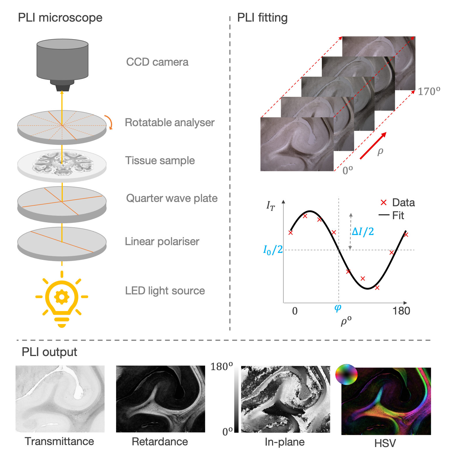
In its most basic for, the PLI microscope is made of three components:
Optics to prepare the polarisation
The thin tissue sample (~50-100 μm thick)
The rotatable analyser and camera
Light from an LED polariser is first shone through a linear polariser and a crossed quarter wave-plate to generate circularly polarised light. The circularly polarised light is then transmitted through the tissue sample where birefringent material results in circular -> elliptical polarisation. Images are then acquired as the analyser (a second linear polariser) is rotated in discrete steps from ρ = 0-180o.
PLI outputs
A sinusoid is fitted to the measured intensity at each pixel (I) as a function of analyser rotation ρ
I = I0 / 2 (1 + sin(2ρ − 2φ) sin δ)
Maps of transmittance, retardance, and in-plane angle were derived from the sinusoid phase and amplitude.
The transmittance, I0, is twice the average intensity of light at the detector and is related to the amount of light extinguished by the sample.
The retardance, ΔI = |sin δ|, describes the ellipticity of the polarisation and is determined by both the quantity and birefringence of myelin, as well as its orientation (inclination) with respect to the imaging plane.
The in-plane angle, φ, describes optic axis which is assumed to align with the azimuth or in-plane angle of the fibre.
To aid interpretation, a composite hue-saturation-value (HSV) image is generated where the hue is defined by the in-plane angle and the value given by the retardance.
In BigMac, we also estimate a proxy inclination map α from δ = C cos2 α, where C is set to some constant value based on a previous study (Mollink2017). As the value of C used is likely highly inaccurate, these maps should not be quantitative. In BigMac, these maps are solely used for co-registration of the PLI and MRI data.
Interpreting retardance
A low PLI retardance can be associated with multiple microsturctural features including the presence of crossing fibres within a single pixel (where each fibre has equal and opposite affect on the PLI signal), fibres having a high inclination angle with respect to the microscopy plane, tissue processing and the amount of time between coverslipping and imaging, or there being a low density of myelin in the tissue. Consequently, care should be taken when comparing retardance values across regions.
Myelin-stained histology
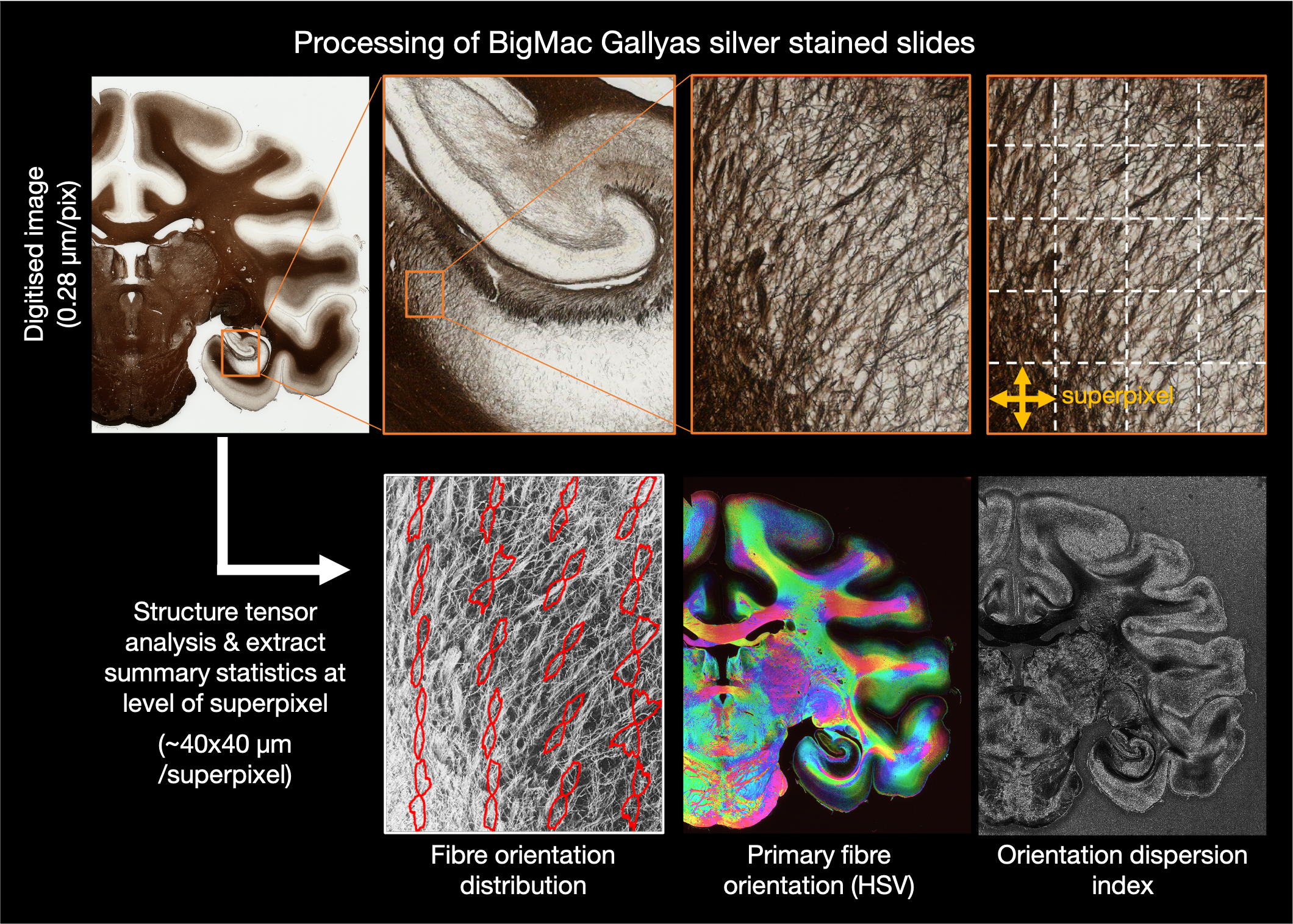
A different set of tissue sections (also 50 μm thick) were stained using Gallyas silver to visualise myelin. The Gallyas silver stains myelin brown, where the sections were then digitised using an Aperio slide scanner with a 20x/0.75 NA objective lens and a 2x magnification lens, to give a resolution of 0.28 μm/pixel. Due to the large slide size, many of the central sections were digitised in two images (labelled image ‘a’ and ‘b’).
Interpreting staining densities
Though the density of the stain carries useful information, using the “stain density” as a quantitative metric can be problematic for several reasons: 1) it may not be linearly related to the amount of myelin present and 2) there can be staining differences between slides, meaning that it is difficult to compare staining densities across slides. Consequently, we would recommend either extracting the stained area fraction from the myelin slides (processed maps coming soon), or thinking carefully about how to combine staining densities across slides.
Structure tensor analysis
The digitised images were subsequently processed using structure tensor analysis (Bigun2005, Budde2012) to estimate the primary fibre orientation per pixel. Here we use a Gaussian kernel of 10 μm and estimate summary metrics over a local neighbourhood (superpixel) of 150x150 pixels, which is approx 40x40 μm. The summary metrics include:
HSV - the colour coded mean orientation weighted by the staining density
Orientation - the mean in-plane fibre orientation across the superpixel
RBG thumb - mean RGB value for superpixel
FOD - the fibre orientation distribution - a frequency histogram of all fibre orientations within the super pixel.
Key references:
Mollink, J., Kleinnijenhuis, M., van Cappellen van Walsum, A.M., Sotiropoulos, S.N., Cottaar, M., Mirfin, C., et al. Evaluating fibre orientation dispersion in white matter: Comparison of diffusion MRI, histology and polarized light imaging. NeuroImage 2017;157:561{574. doi:10.1016/j.neuroimage.2017.06.001.
Axer, H., Axerl, M., Krings, T., Keyserlingk, D.G.v.. Quantitative estimation of 3-D fiber course in gross histological sections of the human brain using polarized light. Journal of Neuroscience Methods 2001;105(2):121{31. doi:10.1016/S0165-0270(00)00349-6.
Larsen, L., Gri n, L.D., Gra el, D., Witte, O.W., Axer, H.. Polarized light imaging of white matter architecture. Microscopy Research and Technique 2007;70(10):851-863. doi:10.1002/jemt.20488.
Axer M, Amunts K, Grässel D, Palm C, Dammers J, Axer H, Pietrzyk U, Zilles K. A novel approach to the human connectome: ultra-high resolution mapping of fiber tracts in the brain. Neuroimage 2011; 15;54(2):1091-101. doi: 10.1016/j.neuroimage.2010.08.075.
Axer, M., Grassel, D., Kleiner, M., Dammers, J., Dickscheid, T., Reckfort, J., et al. High-Resolution Fiber Tract Reconstruction in the Human Brain by Means of Three-Dimensional Polarized Light Imaging. Frontiers in Neuroinformatics 2011;5:34. doi:10.3389/fninf.2011.00034.
Gallyas, F.. Silver staining of Alzheimer’s neuro brillary changes by means of physical development. Acta Morphologica Academiae Scientiarum Hungaricae 1971;19(1):1-8.
Bigun, J., Bigun, T., Nilsson, K.. Recognition by symmetry derivatives and the generalized structure tensor. IEEE Transactions on Pattern Analysis and Machine Intelligence 2004;26(12):1590{1605. doi:10.1109/tpami.2004.126.
Budde, M.D., Frank, J.A.. Examining brain microstructure using structure tensor analysis of histological sections. NeuroImage 2012;63(1):1{10. doi:10.1016/j.neuroimage.2012.06.042.