Analysis Pipeline Practical

In this practical we will learn how to combine the FSL tools to perform an analysis pipeline, which can be run across a large number of subjects. As an example, we will be reconstructing a version of the FSL VBM pipeline, which we saw earlier in the course as part of the structural MRI practical.

This pipeline will use the `file-tree` and `fsl-pipe` tools included in the FSL package. The `file-tree` tool is used to define a directory structure for the analysis, and the `fsl-pipe` tool is used to run the analysis pipeline. These tools have been implemented in Python. If you are not familiar with Python, you can still follow along with the practical. However, implementing your own analysis pipeline in Python will require some knowledge of the language.

Implementing your analysis pipeline in `fsl-pipe` has many advantages over using a shell script:

You can run the same pipeline locally or in parallel on a computing cluster.
The pipeline can intelligently only run the bits that are needed in case you re-run it.
You can easily switch between running a few test subjects and the full pipeline.
Each part of the pipeline is clearly delineated with its own inputs or outputs, which makes it easier to add or edit individual jobs.
You can request a specific output file and the pipeline will only run the jobs needed to produce that output file.

Exploring the input data.: Use `file-tree` and `fsleyes` to visualise images across many subjects.
Adding a first job to the pipeline.: Add your first brain extraction job to the pipeline using `fsl-pipe` and `file-tree`. The output is visualised again using `fsleyes`.
Adding a second job to the pipeline.: Adds a segmentation job to the pipeline. Explore how to deal with the main output files produced by many FSL commands such as `fast`.
Adding registration jobs to the pipeline.: Expanding the pipeline with two more jobs for linear and non-linear registration.
Building a template.: Explore how to add jobs to the pipeline that do not run in parallel across all subjects.
Adding a final job to the pipeline.: Explore how to use both subject-specific and template input files for your pipeline jobs. We also visualise the full pipeline as a graph.
Running the pipeline on a computing cluster.: Transfer the pipeline from your local computer to a computing cluster.
Final words: Briefly describes some additional `file-tree` and `fsl-pipe` features and points to additional sources of documentation.

Exploring the input data.

The input data for this practical is the same set of T1-weighted structural MRI images as seen in the structural MRI practical. However, the input data is in a different directory structure. Rather than having a single directory with all the images, the input data is in a directory structure that is more typical with separate directories for each subject.

cd ~/fsl_course_data/pipeline

The input data is in the `input` directory. To explore the directory structure, you might want to open the `input` directory in a file browser. In short, it contains a subdirectory for both patients and controls. Each of these contain subdirectories for each subject, which contains a single T1-weighted structural MRI image in NIfTI format.

The first step of writing a pipeline is to describe this input directory structure to the computer in the `file-tree` format. We will do this as a simple text file, which is already provided called `data.tree`. This file contains the following text:

input
    group-{group}
        sub-{subject}
            group-{group}_sub-{subject}_T1w.nii.gz (T1w)

The indentation in the text file is important. The first line describes the top-level directory, which is `input`. The second line describes the next level subdirectory, which is `group-{group}`. The part between curly brackets will be replaced with the actual group name (i.e., `patient` or `control`). Similarly, the third line describes the next level subdirectory, which is `sub-{subject}`, where the part between curly brackets will be replaced with the actual subject ID. Finally, the last line describes the actual image file, which is `group-{group}_sub-{subject}_T1w.nii.gz`. Once again, the part between curly brackets will be replaced with the same group name and subject ID as used in the subdirectory names. The `(T1w)` gives a short-hand name for this file, which will be used in the analysis pipeline.

Let's have a look at the data using `fsleyes`.

fsleyes &

We want `fsleyes` to understand the directory structure we just described. To do this, follow these steps:

Click on the "Settings" button in the menu bar followed by "Ortho View 1" and tick the box "File tree". This will open a new menu on the right-hand side of the screen
Ensure that the selected file-tree in the top of this menu is "data.tree". If it is not, you can load this file using "Load tree file".
Select "Load directory" and select the directory you are currently in (i.e., `~/fsl_course_data/pipeline`). This will add a checkbox on the left with the label "T1w" (matching the short-hand name we used in the `data.tree` file).
Click on the checkbox to load the data.

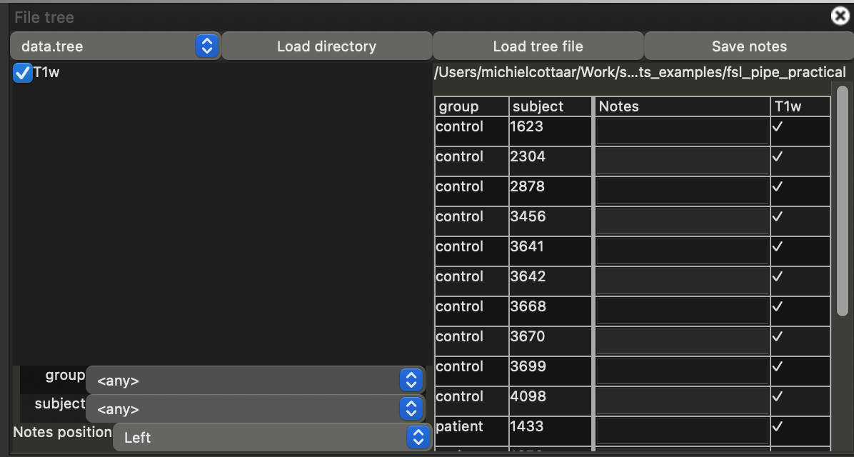
This will result in a view similar to the one below:

Note that a table has appeared with the subject IDs and group names. You can click on any table row load the corresponding T1w images in the main window. Note that any adjustments you make to the view (e.g., adjusting the maximum brightness) will be retained when you select a different subject. You can also switch between subjects using the "up" and "down" arrow keys on your keyboard.

Now that we have explored the input data, we can start writing the analysis pipeline.

Adding a first job to the pipeline.

We have already written the boilerplate code to set up the analysis pipeline for you in the file `pipe.py`. When writing an analysis pipeline using `fsl-pipe`, we will be regularly updating both this file and `data.tree`. So, it is a good idea to open both files next to each other in a text editor. Lastly, you will need to open a terminal window to run the analysis pipeline. Running the pipeline is done using the command:

fslpython pipe.py

For now, running this command will result in an error message, because we have not yet added any jobs to the pipeline. The first job we will add to the pipeline is the `bet` command, which is used to extract the brain from the T1w images. Our first step will be to define, where the output of the `bet` command will be saved. We will here follow the good practice of saving the output in a separate directory, which is called `output`. Let's add this directory to the `data.tree` file. Add the following lines to the end of the `data.tree` file:

output
    group-{group}
        sub-{subject}
            T1w_brain.nii.gz

Next we will add the `bet` command to the pipeline. To do this, we will add the following lines to the `pipe.py` file. You can add these just after the line that says `# Filled by user`:

@pipe
def brain_extract(T1w: In, T1w_brain: Out):
    wrappers.bet(T1w, T1w_brain)

The `@pipe` decorator is used to define a new "recipe" in the pipeline. The recipe itself is defined as a regular Python function, which takes two arguments: `T1w` and `T1w_brain`. The `In` and `Out` decorators are used to define, which of these files are the input or the output of the recipe. Within the recipe function, we call the `wrappers.bet` function to actually run the `bet` command. Note that this single recipe represents multiple jobs within the pipeline as this recipe will be run for each subject in the input directory structure. During each run, the `T1w` and `T1w_brain` arguments will be replaced with the actual input and output files for that specific subject.

Let's now run the pipeline to see if everything is working. In the terminal, run the following command:

fslpython pipe.py

The pipeline should iterate over all the subjects and groups in the input directory structure and run the `bet` command on each of the T1w images. The output will be saved in the `output` directory structure we just defined. If you encounter any errors, please check the `pipe.py` and `data.tree` files for typos. For reference, you can compare with these pipe.py and data.tree files.

Now that we have run the `bet` command, we can check the output. To do this, we will use `fsleyes` again. If you have the same `fsleyes` window open as before, you can simply select "Load tree file" and select the updated `data.tree` file. This will add a new checkbox on the left with the label "T1w_brain". Click on the checkbox to load the data. In the main image window, there will now be two images loaded: the original T1w image and the brain-extracted T1w image. Please, ensure that the brain-extracted image is on top and change the color map to "Red-Yellow".

As you flip through the subjects using the "up" and "down" arrow keys, you can now see the quality of the brain extraction. The brain extraction clearly failed for most subjects with a large amoung of neck included in the brain mask. This is because the `bet` command is not very good at extracting the brain from T1w images with a lot of neck included. It illustrates the importance of checking the output of each step in the pipeline rather than just assuming that everything is working. `File-tree` in combination with `fsleyes` is a great way to do this.

If you want to learn more about using `file-tree` in `fsleyes`, you can check out the documentation here.

Let's fix the brain extraction in the matter done with the FSL VBM pipeline. Within VBM this is done in a three-step process:

First, `bet` is run with the default settings, even though this includes a lot of neck.
This flawed masked brain image is registered to standard space, so that we can use the standard brain mask cut the neck from the image. This is done using the `standard_space_roi` command.
Finally, the `bet` command is run again on the cut image.

We will implement this in the pipeline by editing the first job to read:

@pipe
def brain_extract(T1w: In, T1w_brain_first_attempt: Out, T1w_cut: Out, T1w_brain: Out):
    wrappers.bet(T1w, T1w_brain_first_attempt)
    run(["standard_space_roi", T1w_brain_first_attempt, T1w_cut, "-roiNONE", "-altinput", T1w, "-ssref", f"{getenv('FSLDIR')}/data/standard/MNI152_T1_2mm_brain"])
    wrappers.bet(T1w_cut, T1w_brain, fracintensity=0.4)

Note that this job uses multiple intermediate output files. We will need to define where these files will be saved in the `data.tree` file. Add the following lines to the `data.tree` file:

T1w_brain_first_attempt.nii.gz
T1w_cut.nii.gz

These files need to be produced for each subject, so we need to add them to the `subject-{subject}` subdirectory in the `output` directory. The final `data.tree` file should look like this:

input
    group-{group}
        sub-{subject}
            group-{group}_sub-{subject}_T1w.nii.gz (T1w)
output
    group-{group}
        sub-{subject}
            T1w_brain_first_attempt.nii.gz
            T1w_cut.nii.gz
            T1w_brain.nii.gz

You can, also, compare the final `pipe.py` file with the solution.

Let's run the pipeline again to see if everything is working. In the terminal, run the following command:

fslpython pipe.py --overwrite

Note that we have added the `--overwrite` flag to the command. This is because the pipeline will by default not overwrite the output files if they already exist.

You can again check the output using `fsleyes`. Make sure to load the updated `data.tree` file using the "Load tree file" button. There will be 4 checkboxes on the left (`T1w`, `T1w_brain_first_attempt`, `T1w_cut` and `T1w_brain`). Select three of them for visualisation (`T1w`, `T1w_brain_first_attempt` and `T1w_brain`). If you overlay them in the right order and adjust the color maps (blue for `T1w_brain_first_attempt` and red for `T1w_brain`), you should see the following:

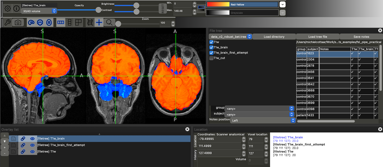
Flip through the subjects to confirm that the new brain extraction is working well.

Adding a second job to the pipeline.

Now that we have a good brain extraction, we can move on to the next step in the pipeline. The next step is to run the `fast` command to segment the brain into different tissue types. We will add this as a second job to the pipeline.

Let's first define where the output of the `fast` command will be saved. The `fast` command produces multiple files. Rather than typing them all out in the `data.tree` file, we can refer to a different `file-tree` that already contains the `fast` output files. This file is available here. Fortunately, it is already installed in FSL, so we can use it directly. To do so, we add the following line to the `data.tree` file (under the output directory, in this example it is `output`):

->fast basename=run_fast (segment)

The `->` symbol indicates that this is a reference to another `file-tree`. The `fast` part indicates that we want to use the `fast` file-tree. The `basename=run_fast` sets the base name used within this `file-tree` (i.e., it fills in the `{basename}` part of the `fast` file-tree). The `(segment)` part gives a short-hand name for all the files within the `fast` file-tree. We can refer to individual files within the `fast` file-tree using `segment/{name within the fast file-tree}`.

Next we will add the `fast` command to the pipeline. To do this, we will add the following lines to the `pipe.py` file:

@pipe
def segmentation(T1w_brain: In, basename: Ref("segment/basename"), gm_pve: Out("segment/gm_pve")):
    wrappers.fast(T1w_brain, out=basename)

The general format is very similar to the `brain_extract` job we defined earlier. We can see that we refer to the `fast` file-tree using the "segment" identifier, e.g., `segment/gm_pve` refers to the `gm_pve` file within the `fast` file-tree.

Another difference is that we are using the `Ref` decorator to refer to the `basename` variable within the `fast` file-tree. The `Ref` decorator is used to refer to a filename that is neither an input nor an output of the job. In this case, the `basename` sets the base name used by `fast`, but it is not actually a file produced by `fast` so we cannot label it as `Out`.

Let's run the pipeline to see if everything is working:

fslpython pipe.py

Again, if any errors arise, please compare your files with the reference `pipe.py` and reference `data.tree`.

Note that even though our pipeline now includes two jobs, it only runs the `segmentation` job. The reason for that is that the `brain_extract` job has already been run and the output files already exist. If we wanted to rerun the pipeline from scratch, we could use the `--overwrite` flag.

The pipeline is getting pretty slow now, because it is running the `fast` command on all the subjects. To speed things up during the pipeline development, we can limit the number of subjects being processed. We can do this by overriding the `subject` placeholder values from the command line. To do this, we can use the `--subject` flag followed by a list of subject IDs. For example, to include only a single control and a single patient, we can run the following command:

fslpython pipe.py --subject 1623 1433

If `fast` is still running, you might want to interrupt it using `Ctrl+C` and run the command above instead. If these particular subjects have already been processed, the pipeline will simply report that and terminate.

You can check the output using `fsleyes` again. Make sure to load the updated `data.tree` file using the "Load tree file" button. There will be additional checkboxes on the left corresponding to the `fast` output files. Each of these will start with the `segment/` prefix. Ensure that the `segment/gm_pve` file actually corresponds to the GM partial volume map as we will be using that one in the rest of the pipeline.

Adding registration jobs to the pipeline.

Now that we have the segmentation, we can move on to the next step in the pipeline. The next step is to register the GM partial volume maps from `fast` to standard space. Hopefully, the procedure for adding more jobs to the pipeline is becoming clear by now. In this case, we add two more jobs to the pipeline:

@pipe
def linear_registration(gm_pve: In("segment/gm_pve"), linear_reg: Out):
    run(["flirt", "-in", gm_pve, "-ref", f"{getenv('FSLDIR')}/data/standard/tissuepriors/avg152T1_gray", "-omat", linear_reg])

@pipe
def nonlinear_registration(gm_pve: In("segment/gm_pve"), linear_reg: In, nonlinear_reg: Out, gm_pve_in_standard: Out):
    run(["fnirt", f"--in={gm_pve}", f"--ref={getenv('FSLDIR')}/data/standard/tissuepriors/avg152T1_gray", f"--aff={linear_reg}", f"--cout={nonlinear_reg}", "--config=bad-fnirt-config.cnf", f"--iout={gm_pve_in_standard}"])

`linear_registration` uses the `flirt` command to perform a linear registration of the GM partial volume maps to the standard space. The resulting affine transformation matrix is saved in the `linear_reg` file, which is used as input to the `nonlinear_registration` job. The `nonlinear_registration` job uses the `fnirt` command to perform a nonlinear registration of the GM partial volume maps to the standard space.

All of these output files need to be defined in the `data.tree` file. For clarity, let's include them into their own subdirectory called `xfms`. Add the following lines to the `data.tree` file (under the output directory, in this example it is `output`):

xfms
    gm_pve2standard.mat (linear_reg)
    gm_pve2standard.nii.gz (nonlinear_reg)
    gm_pve_in_standard.nii.gz (gm_pve_in_standard)

Once again, ensure that these files are included in the `subject-{subject}` subdirectory in the `output` directory. Reference files are available here (`pipe.py`) and here (`data.tree`). Run the pipeline again to see if everything is working for our two test subjects:

fslpython pipe.py --subject 1623 1433

Building a template.

Now that we have the GM partial volume maps in standard space, we can build a template. This job is a bit different from the previous jobs, because it will not be run independently for each subject. Instead, we will run it once for all the subjects. In `fsl-pipe`, this can be done by setting the `no_iter` flag to the placeholders that you do not want to iterate over (i.e., `group` and `subject`). So, the job will look like this:

@pipe(no_iter=["group", "subject"])
def create_template(gm_pve_in_standard: In, gm_pve_template: Out):
    import nibabel as nib
    import numpy as np
    ref_img = nib.load(gm_pve_in_standard.data[0])
    average_gm_pve = np.mean([nib.load(fn).get_fdata() for fn in gm_pve_in_standard.data], axis=0)
    template = (average_gm_pve + average_gm_pve[::-1, :, :]) / 2  # add the flipped image to enforce left-right symmetry
    nib.save(nib.Nifti1Image(template, ref_img.affine, ref_img.header), gm_pve_template)

Note the use of the `no_iter` flag after the `@pipe` decorator.

Note that in this job we are using the `nibabel` library to load and save NIfTI images instead of the `FSL` command line tools. This is to illustrate that you can use any Python library within the pipeline. The `nibabel` library is a popular library for working with NIfTI images in Python available here.

In the `data.tree` file, we need to add the output file for the template. In this case, the output file is not subject-specific, so it should not be included in the `subject-{subject}` subdirectory. Instead, we will add it to a `template` subdirectory directly within the `output`. Add the following lines to the `data.tree` file:

template
    gm_pve_template.nii.gz

Use the indentation to ensure that this is a subdirectory of the `output` directory. If necessary, you can compare with the `data.tree` solution. If any errors arise, please also compare your pipeline with the reference `pipe.py`. Run the pipeline as normal for our two test subjects:

fslpython pipe.py --subject 1623 1433

This should only run a single job, which will create the template from both subjects' input data.

Adding a final job to the pipeline.

Let's see how we can use this template on the single subject level again. We will do this in a final job, which will register the subject's GM partial volume map to the template. This job will be similar to the `nonlinear_registration` job we defined earlier. However, this time we will use the template as the reference image instead of the standard space.

The job will look like this:

@pipe
def register_to_template(gm_pve: In("segment/gm_pve"), gm_pve_template: In, linear_reg: In, gm_pve_in_template: Out, gm_pve_jac: Out, gm_pve_mod: Out):
    wrappers.fnirt(gm_pve, gm_pve_template, aff=linear_reg, iout=gm_pve_in_template, jout=gm_pve_jac, config="bad-fnirt-config.cnf")
    wrappers.fslmaths(gm_pve_in_template).mul(gm_pve_jac).run(gm_pve_mod)

Note that the template is a regular input file (marked with `In`) just like any of the subject-specific files. When writing the pipeline, we do not have to distinguish between subject-specific and template files.

In addition to the registration, this job also computes the modulated GM partial volume map using the Jacobian determinant of the warp field.

Add the new subject-specific output files (i.e., `gm_pve_in_template`, `gm_pve_jac`, `gm_pve_mod`) to the `data.tree` file and run the pipeline again for the two test subjects. Reference files are available here (`pipe.py`) and here (`data.tree`).

Let's visualise our complete pipeline. To do this, we will add the `pipe.add_to_graph(tree=tree).render("my_pipeline")` command to the end of the `pipe.py` file. This will create a file called `my_pipeline.svg` in the current directory. You can open this file in a web browser to visualise the pipeline. The pipeline will look something like this:

Each red box represents a job in the pipeline. The blue ovals represent the input and output files for each job. The arrows represent the flow of data between the jobs. For each job and file, the graph also lists the placeholders over which the job is iterated. For example, you can see that only the `create_template` job is not iterated over the `group` and `subject` placeholders.

Running the pipeline on a computing cluster.

Now that we have a working pipeline, we can run it on a computing cluster. In fact, we do not have to change anything in the pipeline to run it on a cluster. When you run the pipeline using the `fslpython` command, it will automatically detect if you are on a cluster and use the appropriate job scheduler. This does require `FSL` to be installed on the cluster including a correct setup of `fsl_sub` (ask your system administrator if you are not sure).

Even though the pipeline will run without any changes, it can be useful to add some additional information to the cluster job scheduler. This can be done by adding a `submit` flag to the `@pipe` decorator. In particular, we will set the maximum run time of each job, using a format like:

@pipe(submit=dict(jobtime=10))
def ...

This will set the maximum run time of this particular job to 10 minutes. Note that this is the run time for a single job (i.e., for a single subject). Let's add these flags to all of the individual jobs. When running the pipeline locally, you hopefully got some idea of how long each job takes. Make sure that the maximum run time is long enough to actually finish the job. Some example run times for each job are:

brain_extract: 3 minute
segmentation: 10 minutes
linear_registration: 3 minute
nonlinear_registration: 10 minutes
create_template: 3 minutes
register_to_template: 10 minutes

In addition, you might want to change the configuration files used in the `fnirt` command. In our pipeline definition above we used `bad-fnirt-config.cnf`, which was designed to run very quickly, but it gives poor results. For a better registration, you can use `GM_2_MNI152GM_2mm.cnf`, which is the recommended configuration file for registering GM partial volume maps.

After these changes your `pipe.py` should look like this. If you have access to a computing cluster, copy the `input` directory and the `pipe.py` and `data.tree` files to the cluster. You can then run the pipeline using the standard command:

fslpython pipe.py

Final words

Congratulations! You have now written a complete analysis pipeline using `fsl-pipe` and `file-tree`. It reproduces most of the FSL VBM pipeline, except for the final merging of the modulated GM partial volume maps and the statistical analysis. The merging can be implemented as an additional job very similar to the `create_template` job. The statistical analysis is a bit more complicated, since it requires a design matrix and a contrast matrix as additional inputs from the user. Adding these features is left as an exercise for the reader.

Both `file-tree` and `fsl-pipe` have many more features than we have covered in this practical. We can explore some of them just by looking at the command line help:

fslpython pipe.py --help

This will give you a list of all the available options for the pipeline. For example, you can select a specific output file to be produced by the pipeline just by listing this file on the command line:

fslpython pipe.py output/group-control/sub-3456/xfms/gm_pve_in_standard.nii.gz --overwrite

This will run the parts of the pipeline that are needed to produce this output file. Note that this will not run the `create_template` job, because it is not required to produce the registration to standard space requested in the command. We could get the same effect by running the command:

fslpython pipe.py gm_pve_in_standard --subject 3456 --overwrite

Here we use the short name defined in the `data.tree` file (i.e., `gm_pve_in_standard`) to refer to the output file. This is equivalent to the `output/group-control/sub-3456/xfms/gm_pve_in_standard.nii.gz` file name.

There are also some additional features in `fsl-pipe` that are not available in the command line. For example, we can use a subset of all subjects in the template creation by adding a list of subject IDs to the `@pipe` decorator of the `create_template` job (e.g., `@pipe(placeholders=dict(subject=[...]))). This replicates the use of `template_list` in the FSL VBM pipeline.

You can find more information about `file-tree` and `fsl-pipe` in the file-tree documentation and the fsl-pipe documentation.

The End.