FSL-MRS Practical

This is the FSL-MRS practical. FSL-MRS is FSL's end-to-end magnetic resonance spectroscopy (MRS) toolbox. FSL-MRS also handles magnetic resonance spectroscopic imaging (MRSI).

Contents:

SVS:

Data Conversion

How to convert raw MRS data to the NIfTI-MRS format.

Data Exploration and Interpretation

How to interpret MRS data in the NIfTI-MRS format.

Pre-processing

Pre-process MRS data, ready for spectral fitting.

Basis Spectra

What's in a set of basis spectra?

Fitting

Fitting the SVS data using FSL-MRS.

Interpreting SVS Fits

Explore the results of SVS fitting in FSL-MRS's interactive report.

MRSI:

Fitting MRSI Data

Fit a pre-processed MRSI dataset.

Exploring the MRSI Results

Visualise the MRSI fit in FSLeyes.

Optional extensions

FSL-MRS can also be used to create a set of basis spectra. In this optional section we will take you through the steps required to simulate your own basis spectra.

Making a JSON Sequence Description

How to correctly populate a JSON formatted sequence description file.

The FSL-MRS Simulator

How run the FSL-MRS basis set simulator, and verify your results.

Adding MM Basis

How to add a macromolecular basis spectrum to your simulation.

The FSL-MRS Pipeline

Data Conversion

MRS data comes in a wide variety of formats. Though MRS data can be stored in DICOM format, it is just as common for MRS data to be exported from the scanner in a specific vendor format (for example .dat 'twix' for Siemens, p-files for GE, or .SDAT/.SPAR for Philips). One reason for this is DICOM MRS does not provide an intuitive, or standardised way to store data which has two or more dynamically changing parameters, for example individual coil elements or dynamic scans, both of which are important in MRS research. The upshot is that data comes in a bewildering range of formats which need dedicated interpretation. Alongside FSL-MRS we have developed a tool spec2nii to convert many different types of MRS data to a new standard known as NIfTI-MRS. In this section, we will use spec2nii to convert some Siemens MRS data to the NIfTI-MRS format.

In this practical we will use data from a Siemens 7T MRI scanner. The data was acquired using a single voxel (SVS) 'STEAM' sequence from a healthy volunteer. The data was exported using the Twix interface and then subsequently downloaded from the scanner.

In this section we will use spec2nii to first investigate what is in the exported files, and then perform the conversion to NIfTI-MRS. In the subsequent section we will look closer at the data and associated meta-data.

Data contents

Navigate to the relevant folder containing the SVS data and take a look at the contents.

cd ~/fsl_course_data/fsl_mrs/svs
ls -la *.dat

You should see two files with complex alphanumeric file names. One file contains data where water suppression is used "...STEAM_metab_FID..." and one file where water suppression is not used "...STEAM_wref_FID...". The latter file contains the water reference data and will be used to pre-process the former file (and eventually for concentration scaling).

We will now use spec2nii to examine what the data contains. We do this using the twix mode and the -v flag.

spec2nii twix -v meas_MID310_STEAM_metab_FID115673.dat

spec2nii has loaded the data and reported on the command-line the contents of the file. You will see that this particular file contains two sets of data labelled image and phasecor. These are Siemens specific tags. The first two dimensions Col, Cha of both image and phasecor are identical in size (4096, 32). These correspond to the spectral time-domain and the number of RF receive coils. The additional set dimension of image is used to store temporal averages, and in this instance we use our knowledge and intuition (because there are 64 temporal averages) to know we want to extract the image data. The phasecor tag contains some built-in water reference data that this sequence includes. We are going to ignore this and use the data contained in the other file, but in a pinch this extra data would do.

Conversion

Now we know what our data contains we want to convert the correct bits. We run spec2nii again to do this. Once again we will use the twix mode but specify -e image and a name and location to output the converted data -f steam_metab_raw -o.

spec2nii twix -e image -f steam_metab_raw -o data meas_MID310_STEAM_metab_FID115673.dat

The output should report that data of size (4096, 32, 64) has been found and that the file has been validated. We now repeat this for the other piece of water reference data. Remember to change the output file name. After running the second conversion take a look at what the data directory contains.

spec2nii twix -e image -f steam_wref_raw -o data -q meas_MID311_STEAM_wref_FID115674.dat

ls data/

You should see the two files with you converted with a .nii.gz extension. Conversion is now complete, let's examine the data now it is in NIfTI-MRS format.

Data Exploration and Interpretation

FSL-MRS and spec2nii have command-line tools to examine the contents of NIfTI-MRS files. We will use both the FSL-MRS tool mrs_tools and spec2nii now. Later we will also cover how equivalent exploration can be done interactively in FSLeyes.

Examining NIfTI-MRS files

To get a very quick summary of the data run mrs_tools info.

mrs_tools info data/steam_metab_raw.nii.gz

You should see the data size, dimension tags and some key metadata printed. The size should be (1, 1, 1, 4096, 32, 64). The first three dimensions refer to the spatial x, y, and z directions. This data is SVS, so 1*1*1(=1) makes sense. The fourth dimension is the time domain, containing the FID or echo. The purpose of the last two dimensions are indicated by the dimension tags (up to three can be specified for a maximum of seven dimensions). In this data the tags are DIM_COIL (32), DIM_DYN (64) conveying the fifth dimension contains uncombined receive coils, and the sixth dimension is temporal averages. A list of all the possible dimension tags is available at the NIfTI-MRS standard repository.

The metadata displayed indicates the:

• spectrometer frequency (in MHz),
• the dwelltime (time between points in the time domain) which is the inverse of spectral bandwidth
• the resonant nucleus (indicated here as proton by "1H")
• the scanner field strength (in tesla).

spec2nii dump data/steam_metab_raw.nii.gz

This dumps all the contained metadata to the command line. spec2nii extract can extract all the metadata to a JSON file, which can then be modified and reinserted using spec2nii insert.

Visualising NIfTI-MRS files

We can also visualise the data using mrs_tools vis. This command-line visualiser applies some automatic pre-processing to present a sensible view of the data.

mrs_tools vis data/steam_metab_raw.nii.gz

By default this will coil combine and average the data across both of the higher (fifth and sixth) dimensions. If say we want to view all the transients (only running coil combination) we can use the following command.

mrs_tools vis --display_dim DIM_DYN --no_mean data/steam_metab_raw.nii.gz

There are quite a few temporal averages so this isn't a particularly useful view, but we could split up the file and view only a few temporal averages. mrs_tools split split the file across a specified dimension, it produces two files, the second contains any indices we specify on the command line (the first contains all the others).

mrs_tools split --file data/steam_metab_raw.nii.gz --dim DIM_DYN --indices 0 19 39 59 --filename tmp
mrs_tools vis --display_dim DIM_DYN --no_mean tmp_selected.nii.gz

Zoom in on the peak at 2.0 ppm using the buttons at the bottom of the window that has appeared. Looking closely you can see each of the coil-combined spectra don't line up exactly. Correcting this is a major aim of the pre-processing in the next section.

Pre-processing

Pre-processing SVS data involves multiple steps. In this workflow we will apply the following steps:

1. Take averages of water references for use in coil combination of all files.
2. Coil combine the water suppressed metabolite data using the water reference data.
3. Phase and frequency align the data where there are multiple temporal averages.
4. Combine data across those temporal averages by taking the mean.
5. Run eddy current correction using the water reference.
6. In this data an additional FID point is collected before the echo centre. Remove this point.
7. Run HLSVD on the data to remove the residual water in the water suppressed data.
8. Phase the data by using a single peak.

Each of these steps are detailed in the following sub-sections. We'll go into detail in each one as to why they are being run.

The overall aim of the pre-processing is to end up with a single water-suppressed 'metabolite' spectrum and a single water-reference spectrum. Both should have been processed in a near identical way to preserve the relative scaling between them. We therefore must apply processing to take our 32 individual coils and 64 dynamics and produce a single spectrum, appropriately phased, and with the minimum linewidth and maximum SNR possible.

#1. Average the water reference data

We will first tackle the uncombined coil dimension. To do this we will use the high SNR water-reference data to calculate the complex (phase and amplitude) weights needed to appropriately sum each individual coil together. But first, we need to form some water-reference data with an appropriate shape. Our raw water reference data also has a DIM_DYN dimension which needs to be handled for it to be used as a reference. The water signal is high and fairly constant between each element of this dimension so we simply average to collapse the dimension.

For this, and all the other steps in this section we will use the fsl_mrs_proc command. fsl_mrs_proc has a series of sub commands that you will see in turn that apply a single pre-processing operation to a NIfTI-MRS file and return a modified file. In this case we want the average subcommand, and we want to run it on the DIM_DYN dimension of the raw water-reference data data/steam_wref_raw.nii.gz.

fsl_mrs_proc average --file data/steam_wref_raw.nii.gz --dim DIM_DYN --output fsl_mrs_proc --filename steam_wref_tmp

Notice that we have also specified an output file name --filename and output location --output. If you once again run mrs_tools info on the output file you will see that the DIM_DYN dimension has been removed and the shape is now (1, 1, 1, 4096, 32). ^*Reveal command

mrs_tools info fsl_mrs_proc/steam_wref_tmp.nii.gz

#2. Coil combination

Now that we have formed our reference for coil combination we will use it to combine the metabolite water-suppressed data, and the water-reference data itself. We call the coilcombine function of fsl_mrs_proc to do this, providing the previously formed data as a reference. The wSVD algorithm will then be run, combining data and removing the DIM_COIL dimension.

fsl_mrs_proc coilcombine --file data/steam_metab_raw.nii.gz --reference fsl_mrs_proc/steam_wref_tmp.nii.gz --filename steam_metab_comb --output fsl_mrs_proc -r
fsl_mrs_proc coilcombine --file data/steam_wref_raw.nii.gz --reference fsl_mrs_proc/steam_wref_tmp.nii.gz --filename steam_wref_comb --output fsl_mrs_proc

In the first call above notice that we provided the -r flag. This requests that fsl_mrs_proc produces an HTML report on the step. All fsl_mrs_proc commands can produce their own report, which we can then combine together to form a single complete pre-processing report. We'll see how to do that later.

Try opening the coil-combination report now in a browser window. This command can be run after each step to (re)open the reports which generated after each step of pre-processing. The reports are stored in the fsl_mrs_proc directory and named according to the time they were run.

firefox fsl_mrs_proc/*.html

You will see the results of coil combination on the metabolite water-suppressed data. Notice that the combined signal SNR is much higher than the individual channels, revealing many peaks in the spectrum. For brevity, by default only the result of the first index of the remaining DIM_DYN dimension are shown, to change this you can add the --allreports flag.

#3. Phase and frequency alignment

At this point we now have a single dimension left to deal with in our metabolite and water-reference data: DIM_DYN. As we saw in the spectrum visualisation step above the independent acquisitions that make up this dimension are shifted along the frequency axis, and also have different phase. These shifts mostly arise due to physiological (respiratory and cardiac) effects. In this step we want to use the similarity of each signal to re-phase and shift the spectra back into alignment.

1. Between 0.2 and 4.2 ppm for the water-suppressed metabolite data. This excludes any residual water signal, which might have highly variable phase which is uncorrelated with the phase of the rest of the spectrum.
2. Wide limits, 0 to 9 ppm, are given for the water data as the spectrum is dominated by the water signal, the target for alignment.

fsl_mrs_proc align --file fsl_mrs_proc/steam_metab_comb.nii.gz --ppm 0.2 4.2 --output fsl_mrs_proc -r --filename steam_metab_align --apod 20 
fsl_mrs_proc align --file fsl_mrs_proc/steam_wref_comb.nii.gz --ppm 0 9 --output fsl_mrs_proc --filename steam_wref_align

In addition to the output and report flags, there is one other flag used: --apod 20 standing for apodisation. Apodisation applies a filter to reduce noise (at the expense of broadening peaks). For the alignment it reduces the effect of noise on the optimisation process.

#4. Data averaging

The previous step aligned all the data ready for averaging, but it didn't perform the averaging step. Run mrs_tools info on the output of the last step to check for yourself. In this step we simply call fsl_mrs_proc average again to achieve this.

fsl_mrs_proc average --file fsl_mrs_proc/steam_metab_align.nii.gz --dim DIM_DYN  --output fsl_mrs_proc -r --filename steam_metab_avg
fsl_mrs_proc average --file fsl_mrs_proc/steam_wref_align.nii.gz --dim DIM_DYN  --output fsl_mrs_proc --filename steam_wref_avg

Now look at (visualise) the metabolite data across the full chemical shift range (0 - 6 ppm) after this step reveal command. Three things are apparent about the data:

1. The spectrum is upside down!
2. There is a large residual water peak (a peak at 4.65 ppm with different phase to the others).
3. Less obviously, there are line shape distortions due to the effect of eddy currents. These distortions are most apparent around the base of NAA (at 2 ppm).

mrs_tools vis --ppmlim 0 6 fsl_mrs_proc/steam_metab_avg.nii.gz

#5. Eddy current correction (ECC)

Eddy current correction relies on the high SNR water-reference data experiencing the same eddy currents as the low SNR metabolite data. This is the case if the water-reference acquisition sequence had identical sequence gradients. If the water-reference data experiences eddy current effects we would expect to see a distinctly non-Lorentzian peak shape. Take a look at the averaged water-reference data using mrs_tools vis and answer the following question (you will have to expand the ppm range as above):

We will now use the water reference data to correct the eddy current effects in both the metabolite data and in the water-reference data itself.

fsl_mrs_proc ecc --file fsl_mrs_proc/steam_metab_avg.nii.gz --reference fsl_mrs_proc/steam_wref_avg.nii.gz  --output fsl_mrs_proc -r --filename steam_metab_ecc
fsl_mrs_proc ecc --file fsl_mrs_proc/steam_wref_avg.nii.gz --reference fsl_mrs_proc/steam_wref_avg.nii.gz  --output fsl_mrs_proc --filename steam_wref_ecc

Now compare the water reference data before and after the eddy current correction step and notice the much nicer lineshape. The effect can also be observed on the NAA peak (at 2 ppm) as seen in the most recent report.

firefox fsl_mrs_proc/*.html

#6. Centring the echo

Now we will run that one additional step mentioned above. During data acquisition the signal receive hardware has to be activated at the right time to capture the echo. To ensure that the centre of the echo is captured, and to avoid any artefacts caused by the switching of hardware components it is common to start the signal reception a bit too early. We therefore want to remove any data that we captured and happened before the centre. If we don't do this the spectrum will have first-order phase (a phase linearly dependent on the frequency).

In this data a single point must be removed. This comes from explicit knowledge of the sequence implementation. Other sequences report this correction number in a range of different ways. The lack of consistency in reporting of important meta-data is a frustrating aspect of MRS data analysis, and improving the situation is one aim of NIfTI-MRS and spec2nii.

Once again we treat the water-reference and metabolite data identically.

fsl_mrs_proc truncate --file fsl_mrs_proc/steam_metab_ecc.nii.gz --points -1 --pos first --filename steam_metab_trunc --output fsl_mrs_proc -r
fsl_mrs_proc truncate --file fsl_mrs_proc/steam_wref_ecc.nii.gz --points -1 --pos first --filename steam_wref_trunc --output fsl_mrs_proc

Here we are removing a point --points -1 from the first time points --pos first. You can use mrs_tools info to see the effect of this truncation on the data dimensions.

Note that the visual improvement might be hard to see until phase correction (step #8) has been run.

#7. Residual water removal

Back to our list of remaining steps.

We will now deal with that residual water peak. HLSVD is an algorithm that fits multiple lorentzian peaks to an MRS spectrum. We can use this in a restricted frequency range and 'delete' any peaks in that range.

fsl_mrs_proc remove --file fsl_mrs_proc/steam_metab_trunc.nii.gz --output fsl_mrs_proc -r --filename steam_metab_hlsvd

Hopefully it is clear why we don't repeat this step to delete the water signal from the water-reference data ;-).

Use mrs_tools vis to look at the metabolite spectra before and after this step.

#8. Phase correction

Our final preprocessing step is to apply phase correction. This will put the spectrum into a purely positive absorptive mode. I.e. all the singlet peaks should be positive and have no zero-crossings. We run fsl_mrs_proc phase on both bits of data to form our final pre-processed files. For the water-reference data the algorithm is directed just to run phase correction using the water peak between 4.6 and 4.7 ppm (--ppm 4.6 4.7).

fsl_mrs_proc phase --file fsl_mrs_proc/steam_metab_hlsvd.nii.gz --output fsl_mrs_proc -r --filename metab
fsl_mrs_proc phase --ppm 4.6 4.7 --file fsl_mrs_proc/steam_wref_trunc.nii.gz --output fsl_mrs_proc -r --filename wref

Creating a pre-processing report

Now merge the individual HTML reports in the fsl_mrs_proc directory into a single pre-processing report. Simultaneously we will delete all the individual reports, using --delete.

merge_mrs_reports -d "FSL-MRS pre-processing practical." -o fsl_mrs_proc --delete fsl_mrs_proc/report*.html 

If at any point you ran a command twice two reports will have been generated. Both reports will appear in the merged report. (Manual editing can be carried out by deleting the repeated HTML file). Now open the report and look at the last few stages we have run.

firefox fsl_mrs_proc/mergedReports.html

Run through this checklist. Hopefully the answer is yes to all of the questions!

1. Is the metabolite spectrum shown in the penultimate figure the correct way up?
2. Has the residual water peak been removed?
3. Have the eddy current distortions been removed from both spectra? This should be most obvious in the water-reference data in the final figure (compare this to before ECC with mrs_tools vis).

A shortcut for SVS data

Running all those steps was quite hard work. FSL-MRS pre-processing was designed to be flexible and tunable by the user. It would be quite easy to take this practical and formulate your own pre-processing bash script. However, for standard SVS data FSL-MRS also has a packaged processing pipeline fsl_mrs_preproc. The below command should run a very similar set of pre-processing steps from a single command-line call. Try it and compare the reports generated.

fsl_mrs_preproc\
      --output fsl_mrs_preproc\
      --data data/steam_metab_raw.nii.gz\
      --reference data/steam_wref_raw.nii.gz\
      --hlsvd\
      --leftshift 1\
      --t1 T1.nii.gz \
      --overwrite --report

Next we will take a quick look at basis spectra before moving on to fitting this pre-processed data.

Basis Spectra

In the previous section we have pre-processed the supplied data. We therefore have the metabolite water-suppressed data that we will take forward to fitting, and we also have the water-reference data for scaling the concentrations after fitting. One further thing is needed for fitting: basis spectra. For this dataset we have supplied a pre-calculated set of basis spectra for you to use. The last optional section of this practical goes into more detail on how to create your own basis spectra.

You can visualise the basis spectrum supplied using the mrs_tools vis command. Do this now and take a look at the collection of different metabolite basis spectra.

mrs_tools vis steam_11ms

You should see a figure with twenty different spectra. Most contain narrow lines, these are the 19 different metabolites (small biologically active molecules) contained in this set. These have all been simulated using known descriptions of the chemical structure of the metabolites, combined with the sequence timings.

There is one conspicuously different signal, it contains many broad peaks appearing across the whole spectrum.

This set of basis spectra appears as we would expect it: most signals appearing in between 2.0 and 4.5 ppm, and well phased. We are fine to proceed.

Fitting

We now turn to fitting. This is where we use the set of simulated metabolite spectra that we examined in the previous section, alongside a model, to fit our SVS data.

FSL-MRS has a command-line interface (fsl_mrs) that allows for fitting. Let's begin with a simple call to the program, we need to provide the SVS water-suppressed data, the basis spectra, and an output folder name. Here we will also ask the program to output a HTML interactive report to easily and interactively visualise the output.

fsl_mrs --data fsl_mrs_proc/metab.nii.gz \
        --basis steam_11ms \
        --output fsl_mrs_fit \
        --report

The fitting should not take too long. After it has finished, open the report in a web browser:

firefox fsl_mrs_fit/report.html

Take a few minutes to look through all the sections in the report. You should be able to interact with all the plots/figures. For example, starting with the spectral fitting (the first plot), try to zoom in and out, toggle the different traces on and off. You should be able to see that the fitting is good within a specific spectral range, but bad outside of this range (hint: use the 'Autoscale' button on the top-right of the plot). This range can be chosen in the command line tool, and what you can see is the default value for this range.

Try also to look at the table and understand the different columns.

Looking at the first table in the report, you may notice that the metabolite concentrations have no units. This doesn't look very quantitative... We do have relative concentrations (relative to total creatine), but ideally we would like to have absolute concentration. For this, we need to use the water spectrum as a reference .

But to get even more accurate absolute concentrations, we need to account for the fact that our single voxel might contain different tissue types with different relaxation properties.

To account for these partial volume effects, usually a T1-weighted structural image is acquired and processed to segment grey/white/csf. This has already been done for you using fsl_anat, which is a script that runs FAST amongst other things.

To provide the fitting script with information on partial volume, we need to run svs_segment. This can take as an input the result of running fsl_anat as well as the SVS data so as to figure out how much partial volume there is in the MRS voxel. Look at the help for svs_segment to figure out how to run it (the diagram below might help). Or click below to reveal the command.

^*Reveal command

svs_segment --anat=T1.anat --output . data/steam_metab_raw.nii.gz

Now you should have a segmentation.json file with the partial volume information. We are ready to do the quantitative fitting. Here is a graph summarising the input/output to the fitting:

Run the command below which implements the graph above:

fsl_mrs --data fsl_mrs_proc/metab \
        --basis steam_11ms \
        --output fsl_mrs_quant \
        --t1 T1.nii.gz --tissue_frac segmentation.json \
        --h2o fsl_mrs_proc/wref \
        --report

Note that we added the H2O data for quantification as well as the tissue fractions. We also included a T1 but that's only used for display in the report. Now let's look at the report.

firefox fsl_mrs_quant/report.html

You should be able to see some new sections in the report, such as the location of the SVS voxel in the brain, information on the volume fractions, and on the water referencing. Importantly, you should be able to see that the concentrations now come with a physical unit (mMol/kg).

Browse through the output folder to see the different output files. In particular, note that all the parameters that are listed as tables in the report are also stored as CSV files for further automated processing.

Interpreting SVS Fits

Let's dive into a little bit more details in the fitting results. For example, we might want to ask how correlated the metabolite concentration parameters are. A high correlation means that, given the data, the metabolites predict very similar looking spectra, and so it is difficult to disentangle them and they might better be considered jointly.

To answer the question above, it is useful to look at the section in the report called "Uncertainty". The matrix shown represents correlations between the various metabolite concentration parameters.

Now let us look at the section called "Individual metabolite spectra". The red traces represent the model prediction of the individual spectra (including the baseline). These are added together to form the full model prediction.

In the legend, double-click on the data. Then single-click on Cr and PCr. Can you see why these metabolites were highly negatively correlated?

At this point you could do several things to refine the fit.

1. If you suspect that there is no sensitivity to a particular metabolite due to very high uncertainty, you could exclude it from the fitting process altogether. For example in this data Ala and Glc have high uncertainty, and they could be exluded by adding --ignore Glc Ala to the call to fsl_mrs.
2. Other peaks apart from Cr&PCr have high negative correlation, particularly PCh and GPC. You can make the results combine these peaks by adding --combine PCh GPC
3. Finally, the baseline could be made more or less flexible, depending on the quality of fit. This can be done by using --baseline_order N where N is the polynomial order used.

Fitting MRSI Data

Now we move on to fitting multi-voxel MRS imaging (MRSI) data. We provide a dataset that has already been preprocessed, and we will only be concerned here with the fitting and visualisation of the results.

cd ~/fsl_course_data/fsl_mrs/mrsi

First let us look at the provided MRSI data. We do this using FSLeyes, which allows us to seemlessly look through different voxels. In the command below, we load FSLeyes with the -smrs flag, indicating that we are using the MRS plugin. We will also load the structural image alongside the data:

fsleyes -smrs T1.anat/T1.nii.gz mrsi.nii.gz

You should see that this is a multi-voxel, single slice dataset. Try to navigate through the different voxels and examine the spectra. You will need to tick the mrsi data in the Overlay list (MRS view panel). Click around in different voxels to get a feel for the overall data quality.

To fit a model to these data, we first need a basis set. There is one provided with this dataset mrsi_basis:

basis_tools info mrsi_basis

We can also visualise the basis set.

basis_tools vis mrsi_basis

This should look like a regular basis set, but you will notice that there is no macromolecule spectrum. The fitting will be pretty bad without those, so we will use the default macromolecule spectrum provided with FSL-MRS, which we will add to this basis set.

We add the default macromolecules using basis_tools add_set --add_MM. However, due to a small issue with frequency conventions that exists in the code currently we have to wrap this command in basis_tools conj. This issue will be fixed in the near future. Once done, the basis_tools conj can be dropped.

basis_tools conj mrsi_basis mrsi_basis_mm
basis_tools add_set --add_MM mrsi_basis_mm mrsi_basis_mm 
basis_tools conj mrsi_basis_mm mrsi_basis_mm

If we look at the modified basis set we will now see several broad peaks added to the right hand side of the spectrum. In the legend these will be labelled as five new basis spectra: MM09-MM21.

basis_tools vis mrsi_basis_mm

Before we start fitting, we need to get partial volume estimates of tissue types, just like we did for SVS fitting. The command line for doing this is very similar:

mrsi_segment --anat=T1.anat --output . mrsi.nii.gz

You should be able to see that unlike for SVS where the output was a single JSON file, here we get 3 NIfTI files (one per tissue type). Load them in the same FSLeyes session and see if they make sense. You should be able to see that they are tissue fractions resampled into the MRSI slice.

We are now ready to run the fitting command. Read the command below and make sure to understand all the different inputs (you can run fsl_mrsi --help to get more details on what the inputs are). The --metab_groups MM09 ... command ensures that each of the macromolecule basis spectra we added above can have its own shift and broadening. The --combine options sum highly correlated metabolites. This may take a few minutes (and up to 10-15 minutes) to run depending on the hardware and number of threads available.

fsl_mrsi --data mrsi.nii.gz  \
         --mask mask.nii.gz \
         --basis mrsi_basis_mm \
         --output fsl_mrsi_out \
         --metab_groups MM09 MM12 MM14 MM17 MM21 \
         --combine Cr PCr \
         --combine NAA NAAG \
         --combine PCho GPC \
         --combine Glu Gln \
         --tissue_frac mrsi_seg_{wm,gm,csf}.nii.gz \
         --h2o wref.nii.gz \
         --report

Once the fitting is done, you can open the report like we did for the SVS data:

firefox fsl_mrsi_out/report.html

This should look familiar. However, you may notice that the report is only telling us about fitting a single spectrum, when in fact we have run it on a number of voxels. The interactive HTML in fact only shows the results of the fitting for the average of all the voxels inside the mask. In the next section, we will look through the results in each voxels using FSLeyes.

Exploring the MRSI Results

If you've already closed FSLeyes, open it again in MRS mode and load the mrsi data alongside the T1:

fsleyes -smrs T1.anat/T1.nii.gz mrsi.nii.gz

Using the menu bar, select Tools->Load FSL-MRS fit and choose the output folder created by the fsl_mrsi command (should be fsl_mrsi_out).

Now you should be able to see a new panel called "FSL-MRS Results" where you can choose which results to display - try selecting a metabolite from the list to view a metabolite map. In the "MRS View" panel you should be able to see the model predictions and baseline. Add the data plot by ticking mrsi in the Overlay list of the MRS View panel on the right. You can look at individual voxels by simply clicking through in the Ortho View panel.

FSLeyes's MRS plugin recognises the different files found in the results folder. You can look at individual metabolite maps (with different types of normalisation/quantitation), you can also look at QC maps (e.g. SNR). Play around and try to familiarise yourself with the output. Compare the fit for high SNR vs low SNR voxels. Compare voxels at the edge of the ROI to voxels in the middle.

End of the main practical.

Carry on for the advanced optional section on basis spectra simulation.

OPTIONAL: Making a JSON Sequence Description

This optional part of the practical will take you through simulation of your own single voxel basis spectra. We will use the FSL-MRS simulator to create a basis spectra set for the STEAM sequence used in the first part of this practical (the SVS data).

To create high-quality basis spectra, the simulator must be provided with an accurate description of the MRS sequence. The description contains:

• the radio-frequency (RF) pulses,
• the slice selection and rephase gradients,
• time delays between pulses,
• information about the voxel size,
• scanner hardware and acquisition information.

cd ~/fsl_course_data/fsl_mrs/basis_creation
cat steam11.json

The JSON file contains the following important fields that we will tackle in turn. For a full reference see the online documentation.

• RF, delays, & rephaseAreas
• CoherenceFilter
• Spatial resolution parameters (x, y, z, resolution)
• B0 & centralShift
• Rx_* parameters
• Other parameters

The STEAM sequence

To understand this file, first we must understand the structure of the STEAM sequence. For reference in this process we have included a schematic STEAM sequence diagram.

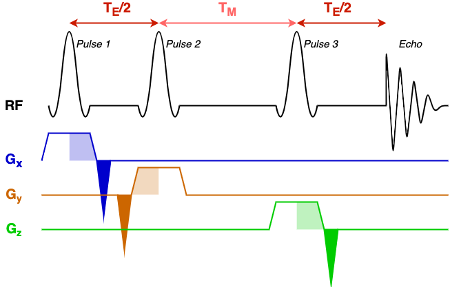
The diagram has a black line denoting RF events (RF pulses and the echo that is formed), and three coloured gradient axes: x, y, and z. In this simple sequence the same 90-degree pulse is repeated three times to form a 'stimulated' echo. Each pulse has an associated slice select gradient, one for each axis, all with the same gradient strength (the voxel has equal dimensions in x, y, and z). Before, or after, the slice-select gradient is a rephasing gradient (dark shaded area) with area equal to half the slice select gradient (light shaded area).

Sequence blocks

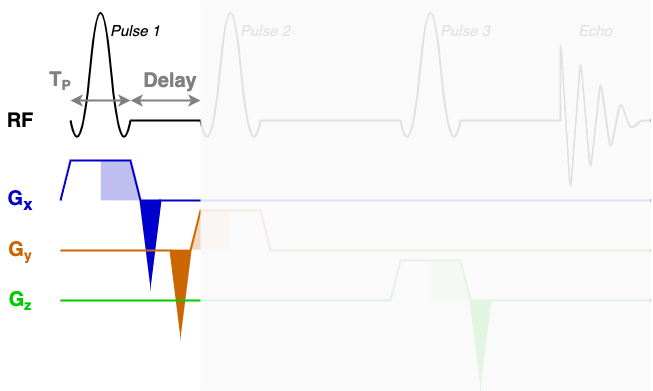
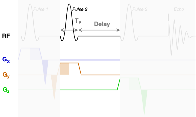
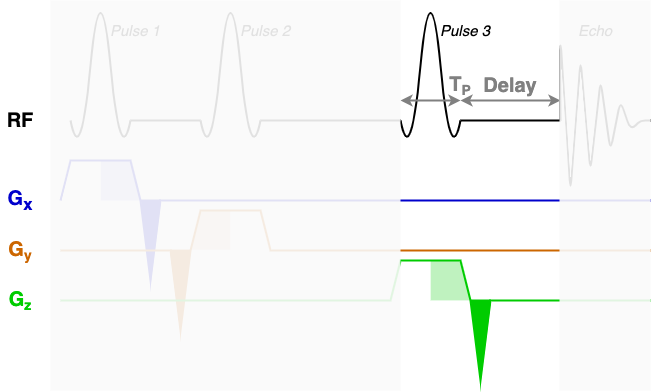
At the core of the sequence description format, an MRS sequence is split up into blocks containing a single RF pulse, associated gradients, and a time delay. The next three diagrams show each of the three sequence blocks in this STEAM sequence. In the sequence description we will describe the RF and gradients in each of the highlighted areas.

RF, delays, & rephaseAreas

Three fields define the majority of the sequence information in the JSON file. These are RF, delays, & rephaseAreas. Try inspecting the packaged sequence description file in a text editor. Take a look at each of those parameters and what data they contain.

You will find that RF contains three blocks of almost identical information. Each block encodes one of the three RF pulses (Pulse 1, Pulse 2, and Pulse 3) using the following fields:

• amp: The pulse amplitude modulation as a list. Typically in units of hertz - a 1 ms hard 90-degree pulse would have an amplitude of 250 Hz.
• phase: The pulse phase modulation as a list. In radians.
• time: The total duration of the pulse (T_P in the diagrams above).
• grad: The slice selection gradient. This is the only field that changes between the blocks, with the constant slice selection gradient iterated over the x, y, and z axes (first, second, and third elements). Typically in units of mT/m.
• frequencyOffset: The frequency offset of the pulse, referenced from the central frequency (see centralShift). In this data the value of -581.2 corresponds to a shift of -2 ppm to centre the pulse in the middle of the spectrum.
• phaseOffset: Fixed phase offset for the pulse, typically 0. In radians.

The delays field is a list with a single delay value per block. In this sequence we have three blocks with three delay times as marked in the figures above.

The rephaseAreas field is a 3 (x, y, z) by N_blocks array. This array encodes the areas of the rephase gradients. During the first block there are two rephase gradients of equal area on the x and y axes([-5.145e-03, -5.145e-03, 0.000e+00]), in the second block there are no rephase areas ([ 0.000e+00, 0.000e+00, 0.000e+00]), in the third block there is a single rephase gradient on the z axis ([ 0.000e+00, 0.000e+00, -5.145e-03]). Note that the areas are negative as the slice selection gradients all have positive magnitude.

CoherenceFilter

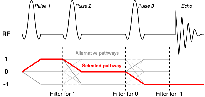
Typically as SVS sequences are repeated to build up temporal averages a series of 'spoiler' gradients are changed incrementally to ensure that unwanted coherence pathways are prevented from appearing in the final averaged spectrum. To copy this approach in simulation would require multiple (tens of) repeated simulations to be run, each with complex gradient structure. Instead FSL-MRS implements a coherence filter to select only the desired coherence pathway.

A discussion of coherence pathways goes beyond this practical, but in brief we want to select a single sequence-dependent pathway from the many that are generated by multiple RF pulses. For STEAM and spin-1/2 systems this corresponds to the [1, 0, -1] pathway. PRESS (with its 90-180-180 RF scheme) would use [-1, 1, -1]. An excellent resource for this is Landheer & Juchem's recent work. For this, and all other, STEAM sequences we set the coherenceFilter field to [1, 0, -1]. This means that after each RF pulse and delay only the coherence in the filter is allowed to proceed.

Spatial resolution parameters (x, y, z, resolution)

For accurate basis spectra, the simulation must be carried out over a fine grid of spatial points, before summation in a final step. We therefore tell the simulation over what spatial grid to simulate. A good recommendation is to set the grid in each dimension (x, y, & z) to twice the voxel size. Here the voxel size was 25 mm isotropic, therefore we set each field to [-25,25] so that simulations take place 25 mm around the centre in each direction (50 mm in total).

The resolution parameter then sets how coarse or fine the grid is for simulation. Always start with a coarse grid (e.g. 5-10) for debugging and tests, as this will speed up the process. A final simulation should be carried out with many points in each direction; in the 40-60 point range.

B0 & centralShift

The B0 parameter sets the main magnetic field strength, this should match the field strength of your scanner. Note that many scanners are not quite the field strength advertised. A 3 tesla scanner might actually be 2.89 T, or a 7 tesla 6.98 T. This information can be found by inspecting the data simulation is being carried out for i.e. mrs_tools info ../svs/data/steam_metab_raw.nii.gz

The centralShift parameter indicates where the central frequency of the scanner was set during any acquisition. Typically, for proton MRS this would be set to the water frequency. Hence to reference between the chemical shift scale - with a somewhat arbitrary zero reference - and the one used experimentally we set this parameter to the chemical shift of water: 4.65 ppm.

Rx_* parameters

There are four parameters which are used to control the appearance of the simulated basis spectra. These are as follows:

• Rx_Points: This controls how many time points will be recorded from the echo in the simulation.
• Rx_SW: This controls the simulated receiver bandwidth (AKA sweep width).
• Rx_LW: The amount of lorentzian broadening applied to the simulated peaks. Should be low (1-2 Hz).
• Rx_Phase: An optional parameter that controls the output phase of the signal. This can be provided automatically by the simulator (see below).

Other parameters

Some of the remaining parameters, sequenceName and description, allow free form text description of the sequence being simulated.

The units parameters: RFUnits, GradUnits, and spaceUnits, allow the user to specify what units some of the parameters are defined in. See the online documentation for more information.

Open up the provided sequence description in an editor and turn down the simulation resolution from [30, 30, 30] to [5, 5, 5]. This should make the next step faster, but more inaccurate; fine for this demo.

OPTIONAL: The FSL-MRS Simulator

Compared to the previous section running the simulator is simple. The simulator is called using fsl_mrs_sim. The user must supply the sequence description and a list of metabolites (or custom described spin systems) to the simulator. The simulator knows about a predefined list of metabolites, meaning the user can just specify their name.

fsl_mrs_sim -b metabs.txt -p -2.0 -e 11.0 -o my_steam_basis steam11.json

In addition to a text list of metabolites supplied in metabs.txt we have added a -p -2.0 flag, a -e 11.0 flag, and -o my_steam_basis. The first automatically phases the spectra (which otherwise would have arbitrary phase) using a peak at -2.0 ppm from the central shift (I.e. 4.65 - 2.0 = 2.65 ppm). The second -e simply adds the echo time to the basis spectra meta-data. The third -o specifies an output location. Try looking at the created basis spectrum, using mrs_tools vis and compare it to the one included in the svs directory.

mrs_tools vis my_steam_basis/
mrs_tools vis ../svs/steam_11ms

The basis should be similar, but differences will arise from the low number of spatial points used to simulate the basis in this practical. Increasing the values in the resolution field to 40 or more would remove any differences, at the cost of greatly increased simulation time.

OPTIONAL: Adding a Macromolecular Basis

Macromolecular basis sets are typically created by empirical measurement of metabolite-nulled spectra. The spectra should be measured using a very similar sequence to the target sequence, in a similar population to the study population, and from a similar anatomical region. The full process is beyond the scope of this practical. However, fsl_mrs_sim can be easily made to incorporate a pre-measured macromolecule basis into one that it is simulating.

Re-run the above command but add -MM macSeed.json. macSeed.json contains a single MM basis spectrum.

fsl_mrs_sim -b metabs.txt -p -2.0 -e 11.0 --MM macSeed.json -o my_steam_basis_with_mm steam11.json

Once again look at the result using mrs_tools vis. The basis set should now contain a MM spectrum.

The End!