FEAT 2 Practical

This tutorial leads you through examples of higher-level group analysis in FEAT.

Paired t-test

We have a group of six subjects, each scanned twice: once doing motor tasks with their left hand, and once with their right hand. This is a stroke study, and hence comparing left and right motor function is particularly interesting in this case. Within each run, subjects completed different blocks of index finger movement, sequential finger movement and random finger movement.

Research question: Is there a significant left vs right hand finger movement paired-difference, generalisable to the population from which the subjects are drawn?

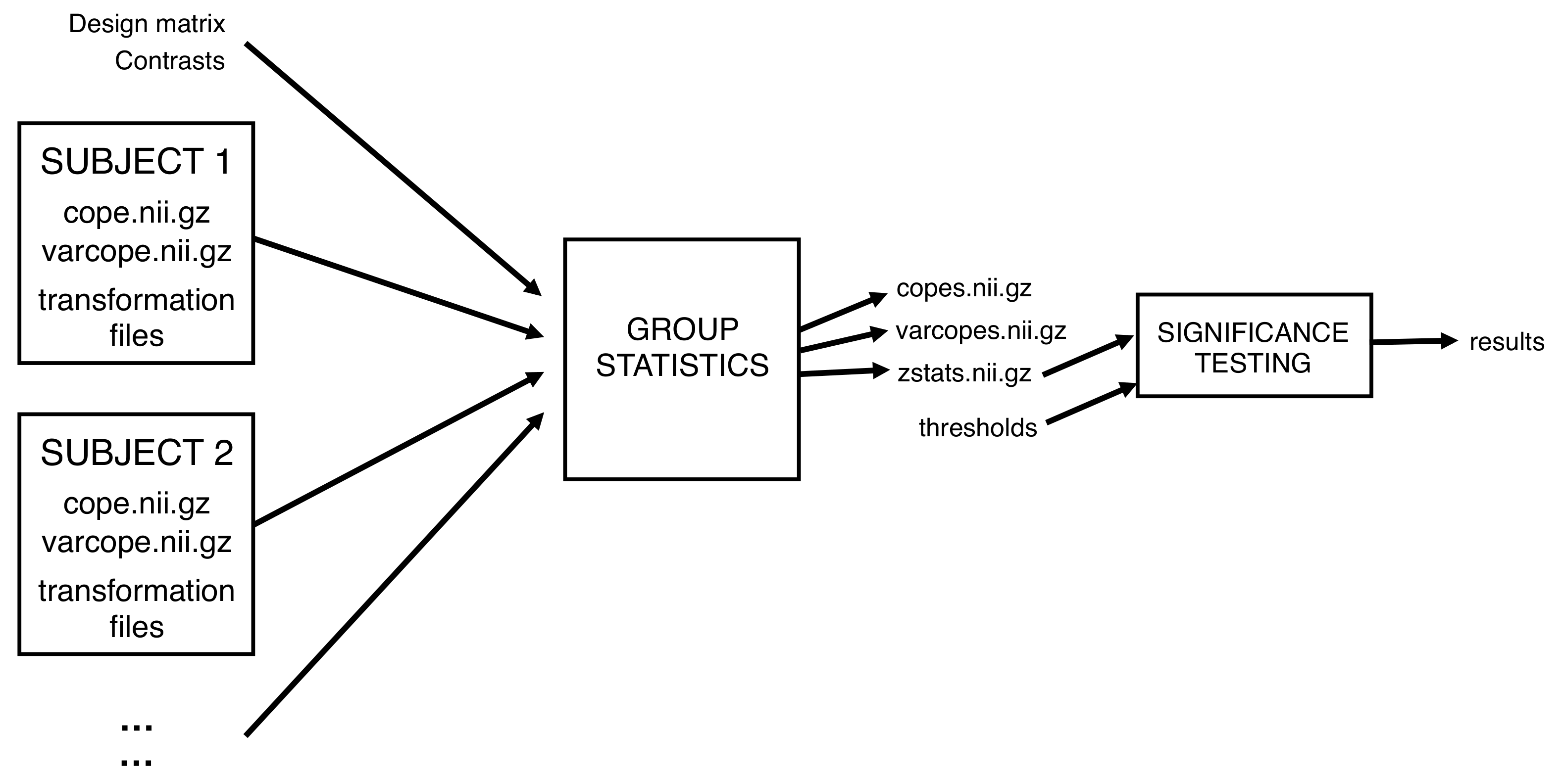
To address this, we want the left − right paired mean difference within a mixed effects model, taking into account the within-subject fixed effects variances and the between-subject random effect variance. This is done as a two-level analysis with the following structure:

Level 1: Single-session analyses There are 6 subjects × 2 sessions = 12 first-level FEAT analyses. These have already been done for you.
Level 2: Between-subject analysis We do a separate second-level analysis for each of the first-level contrasts, and estimate the mean (paired) difference for each.

In FSL terminology, each contrast is represented by a COPE (contrast of parameter estimate), and it is these which we pass up to any higher-level analysis. Note that as well as the COPEs, FEAT passes the variance of these COPEs (VARCOPEs), and even the uncertainty in the variance of these COPEs (DOFs; degrees-of-freedom), between the different levels.

What do the values in a COPE image obtained from the single-session analysis represent?

The parameter estimates for a certain EV Incorrect! COPE (contrast of parameter estimates) images contain combinations of parameter estimates for a certain contrast. For a simple 1 0 contrasts, these may be the same as the parameter estimates for a certain EV, but for more complex contrasts such as 1 -1 these have to be calculated by combining the EV parameter estimates in the correct proportions.
The parameter estimates for a certain contrast Correct! COPE (contrast of parameter estimates) images are calculated by performing simple algebra on the EV parameter estimates. For example, for the contrasts 1 -1, the contrast parameter estimate is calculated by subtracting the parameter estimate for EV 2 from the parameter estimate for EV1. The COPE image will show regions in the brain in which this difference is large.
The uncertainty of the parameter estimates for a certain contrast Incorrect! The uncertainty (or variance) is contained in the VARCOPE image.

First-level analyses

Each first-level analysis contains 6 contrasts, each related to the different types of finger tapping performed in the scanner (e.g. mean response over the different conditions, index finger only, etc.). Thus there are 6 COPEs in the stats subdirectory of each first-level .feat directory. A higher-level FEAT analysis entails an independent analysis on each of these contrasts (i.e. a second-level analysis of all subjects' first-level mean contrasts, a separate second-level analysis of all first-level index contrasts, etc.). Each of these second-level analyses is performed simultaneously and will form a separate cope?.feat directory inside a newly-created .gfeat directory.

cd ~/fsl_course_data/fmri2/paired_ttest

The first-level analyses are held in 6 different directories within ~/fsl_course_data/fmri2/paired_ttest, one for each subject. The subject directories are ac at cm df dn eg. There are two first-level FEAT directories within each of these, and these have already been run for you. Have a quick look at one of the lower-level reports if you want to familiarise yourself with the study design and data.

FEAT set-up

Open FEAT (Feat & or [Feat_gui & on a mac]) and follow the instructions below to set up the higher-level analysis.

First, change First-level analysis to Higher-level analysis in the drop down box at the top.

Data

Here we are going to set up the input data for our higher level analysis. First, change the Number of inputs to 12 (i.e. 6 subjects × 2 sessions).

Press Select FEAT directories. At this stage, you need to decide on a sensible order for the first-level analyses. You could choose to group the analyses by subject (i.e. ac/ac_left.feat, ac/ac_right.feat, at/at_left.feat, etc.), or you could group by condition (i.e. ac/ac_left.feat, at/at_left.feat, …, ac/ac_right.feat, etc.). We recommend the latter option, because this matches the example paired t-test in the FEAT manual, and also matches the way the paired t-test is set up for you if you use the Model setup wizard (explained below).

You can often avoid having to tediously hand-select each of these first-level FEAT directories separately, using the Paste button. If you press this, a new free-text window comes up, within which you can paste text (in this case the list of first-level FEAT directories) which you can copy, e.g. from a list in a terminal. Press Clear to clear the text window. Then in your terminal, making sure you are inside the paired_ttest directory, type:

ls -d1 "$PWD"/??/??_left.feat ; ls -d1 "$PWD"/??/??_right.feat

How does this command work? Answer. This should give you a complete listing of the full pathnames of the FEAT directories in the right order. You can now highlight this list with the mouse, and paste it into the FEAT paste window with the middle mouse button, or by clicking in the paste window and pressing control-y.

ls -1d lists a set of files or directories. The -1 flag prints each result on a separate line, and -d means that only directory names, rather than their contents, are shown. The "$PWD" part fills out the full pathname of the current directory. The ? characters are expanded by the shell to fit any single character, in alphabetical order. The command is repeated so that the _left FEAT directories are listed first, and then all the _right.

To save time, we will only pass the mean contrast up to the top level. Make sure that ONLY contrast 1 is selected in the Use lower-level copes boxes.

When this is done, set the Output directory to paired_ttest_ols (the full path will end up as $HOME/fsl_course_data/fmri2/paired_ttest/paired_ttest_ols.gfeat).

Stats

Select the Mixed Effects: Simple OLS option from the top drop down box. Also, make sure that the Use automatic outlier de-weighting button is NOT turned on. It is important that these two settings are chosen, otherwise the analysis will not be quick enough to be of use to you in the time that we have available for the practical. Normally, we recommend that the more accurate "Mixed Effects: FLAME 1" option is used in combination with outlier de-weighting, for the reasons outlined in the lectures. However, in the interest of speed, in this practical we choose the faster OLS option without outlier de-weighting.

With this design you can use the Model setup wizard, which provides an easy way of setting up a few simple designs. Select two groups, paired and press Process. You will now see the design matrix that has been created for you.

To understand how this is controlled in detail, click on Full model setup.

The inputs (Input 1 to Input 12) correspond to the order you entered the first-level FEAT directories—it is essential that your design matches the order you entered the lower level directories under the Data tab! Note also that the first column, labelled Group, corresponds to groupings of inputs that will share the same random effects (RE) variance in this level of the model. Here, we let all subjects have the same RE variance (i.e. the Group column should be left as all 1s).
There are 7 EVs: EV 1 models the left − right paired difference, and EVs 2-7 are confounds which model out each subject's mean (this is what makes the design a paired t-test).
Click on the Contrasts & F-tests tab. There are two contrasts set up for you by the wizard. EVs 2-7 are confounds of no interest and so do not appear in the contrasts. Hence, the contrasts only involve EV1. Change the Titles boxes to read left > right and right > left.
Press Done.

Post-stats

Because we only use a small number of subjects in order to make it possible to run the analysis in the practical session, we will reduce the cluster threshold slightly. This will allow us to see some more results, but is NOT recommended for your own analyses. In the Thresholding box change the Z threshold to 2.3.

Go!

Press Go! The web browser that appears monitors the overall progress. This second-level analysis should take about 5 minutes. While you're waiting, either make a cup of tea (but do NOT add milk while the bag is still in the water) or familiarise yourself with the introduction to the next major section of the practical on group analyses with multiple sessions per subject.

Results

Higher-level FEAT runs produce .gfeat directories. Once the analysis has finished, explore the web report. This top-level report provides links to the previous level reports, a registration summary page and links to the separate higher-level reports.

LOOK AT YOUR DATA! In particular it is always important to check the registration summary report page very carefully, to ensure that all lower-level registrations succeeded. If any of the lower-level FEATs look like the registration has failed badly, you need to fix this before re-running the higher-level FEAT analysis. Note that field maps were not acquired with this data—you should be able to spot this on the registration page!

In the results page you get a link to the group results from running the group-level analysis on each first-level contrast. Within each contrast you get a group-level results page showing the standard post-stats output. However, note that the time course outputs in these higher-level results no longer refer to time (despite the heading). They refer to subject (or session) number. In this case that is the 12 sessions (6 subjects × 2 conditions) in the study, and it is effect size shown on the vertical axis, rather than normalised MRI signal. Have a look at this and the other parts of the results webpage and make sure you understand what is being shown.

Pre-baked analyses

We have run a full analysis for you on this data (i.e. on all the contrasts, using FLAME for statistics, and with the recommended Z-thresholds). Take a quick look at this report as well.

firefox examples/flame.gfeat/report.html &

Can you spot any major differences between the two analyses?

Group analysis with multiple sessions for each subject

It is common to split a task up into multiple short scans instead of having one long scan. This can often help to reduce subject movement in the scans, and also to keep the attention of your participant. As a result, we need to combine data across multiple scanning sessions using a three-level FEAT analysis.

The data consists of a set of subjects, each scanned twice several months apart. For simplicity's sake, we will look for a simple mean effect across subjects and sessions. Hopefully this will help you understand how this analysis can be extended to more complex questions.

We want the mean group effect, within a mixed effects model, taking into account the within-subject fixed effects variances and the between-subject random effect variance. This is done in THREE levels:

Level 1: Within-session analysis. There are 5 subjects × 2 sessions = 10 of these first level FEAT analyses, which have already been done for you.
Level 2: Between-session analysis. Here, we input the data from Level 1, and estimate each subject's mean response.
Level 3: Between-subject analysis. We input the data corresponding to the subject means from Level 2, model the between-subject variances and estimate the group mean response.

Because each subject will typically only have a handful of sessions, we do not run a mixed effects second-level analysis to get an estimation of each subject's mean response. The reason for this is that we would not be able to get a good estimation of the within-subject session-to-session variance with a limited number of sessions. Hence we choose to ignore the session-to-session variance by using a fixed effects analysis at this second level. See here for a more involved discussion of the choice of a fixed effects analysis.

In addition to this, the analysis cannot be combined into a single second-level analysis. This is tempting as a design matrix can easily be formed containing each subject's mean (across sessions) as a separate EV, and then contrasts can be formed to test the mean across all subjects. The problem with this model is that there are two separate sources of variability (session-to-session and subject-to-subject) but, within FSL, a single level cannot model more than one separate sources of variance.

First-level analyses

In both sessions, subjects performed the "Pyramids & Palm Trees" task (PPTT). Participants are presented with a target image, and are asked to select the image they most associate with the target from a pair of additional images. The canonical example is below:

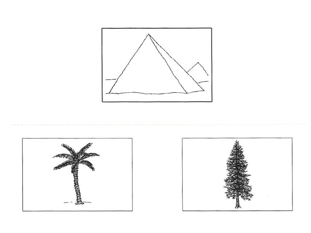
This is meant to be a test of semantic memory, as the task requires reasoning about the links between objects. There is also a control condition, where participants have to match abstract line drawings. We are primarily interested in the semantic > lines responses. To begin with, familiarise yourself with the first-level design and typical responses in one of the session-specific FEAT analyses we have run for you:

cd ~/fsl_course_data/fmri2/3_levels

Take a quick look at one of the web reports within the run directories of the level_1/ directory.

Second-level analysis

We will now set up the second-level (i.e. within-subject) analysis. Open FEAT (Feat & [or Feat_gui & if on a mac]) and follow the instructions below:

Change First-level analysis to Higher-level analysis.
Change the Number of inputs to 10 (5 subjects × 2 sessions).
Press Select FEAT directories. Again, you need to specify the first-level FEAT directories in a sensible order: subject 1, sessions 1, 2; then subject 2, sessions 1, 2; etc. There are lots of ways we can enter these into the GUI: we can enter them individually into the GUI by hand, but this can be laborious for large studies; we can type out the names in a file and use the Paste window; or we could do some simple ls commands and then reorder the outputs as necesary in a text editor. Finally, if we have chosen a sensible naming convention we may be able to script the whole process.

To save time, we will use a command to generate the names we need.

To generate the list, use the command given here.
```
for sub in CON_417 CON_425 CON_428 CON_429 CON_430 ; do
  ls -1d $PWD/level_1/run_1/$sub/*.feat ;
  ls -1d $PWD/level_1/run_2/${sub}_2/*.feat ;
done
```
Note how this command is more complicated than the ones we have used to generate file lists before. This is because of the naming convention we have chosen! Setting up a sensible naming convention from the start will make subsequent analyses immeasurably easier.
Select the text and right-click copy the generated list of names. Paste this text (control-y) in the Paste window.
To save time, we will only pass the semantic > lines and semantic < lines contrasts up to the higher levels. Make sure that ONLY contrasts 1 & 2 are selected in the Use lower-level copes boxes.
Set the Output directory to level_2
Go to the Stats tab and select the Fixed-effects option.
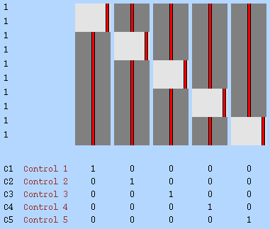
Press Full model setup. Remember that the Inputs (1-10) correspond to the order you entered the first-level FEAT directories. As this is a fixed effects analysis the Group column is ignored so leave all these entries as 1 (if we had lots of sessions and did a mixed effects analysis instead then we would use a unique number in this column for each subject (i.e. within each subject we would estimate a separate variance).
We need 5 EVs: one for each subject mean. Change the 0s to 1s appropriately, in such a way that each EV models a different subject mean. We then need to pass the 5 parameter estimates (PEs) corresponding to the 5 subject means through to the third level as COPEs. To enable this, we need to have a contrast for each subject mean that just selects that parameter. Set the contrasts appropriately. Your design matrix should now match this complete design matrix.
Press Done. The default Post-stats are fine (in fact, the post-stats don't affect what gets passed up to third-level). You are now ready to run the second-level analysis so press Go!

If something has gone wrong with your analysis, or it is taking too long to run, there is a pre-baked version available: examples/level_2.gfeat. You can use this as the input to the third level analysis too if necessary.

This analysis should only take a couple of minutes to run. Wait for the result web pages and then view them carefully. Check that the registrations are accurate, and then take a look at the results.

Third-level analysis

We are now ready to set up the third-level (i.e. between-subject) analysis. This will be valid for one of the contrasts we passed up to the second level (but it is easy to repeat the analysis for the others). We will use the semantic > lines results, which corresponds to contrast 1. Reopen FEAT (Feat &) and follow the instructions below:

Change First-level analysis to Higher-level analysis.
Change Inputs are lower-level FEAT directories to Inputs are 3D cope images from FEAT directories. The inputs will be the 5 COPE images, one for each subject mean, from the second-level analysis.
Change the Number of inputs to 5 (each corresponding to a subject mean).
Press Select cope images and enter the COPEs from the second level. These will be inside the cope1.feat/stats directory which is inside the second-level level_2.gfeat directory that you just created. The relevant command for pasting is:
```
ls -1d "$PWD"/level_2.gfeat/cope1.feat/stats/cope?.nii.gz
```
What does the cope1.feat/stats/cope5.nii.gz represent?

The mean for subject 1 for the fifth contrast that was entered at the first-level analysis Incorrect! The cope1.feat directory contains the results for the first contrast at the subject level, which in this case is semantic > lines.
The mean for subject 5 for the first contrast that was entered at the first-level analysis Correct! The cope1.feat directory contains the results for the first contrast at the subject level, which in this case is semantic > lines. Within that directory, the individual cope5.nii.gz files represent the second-level contrasts, which in our case correspond to individual subjects.
The third group-level statistical result for the first contrast that was entered at the first-level analysis Incorrect! These are the results from the second-level analysis, so this is an average for an individual subject (specifically in this case for subject 5)
Set the output directory to level_3
Go to the Stats tab and change to Fixed effects. Note that this is NOT recommended for group-level analyses, but we use it here to save time and because we are only analysing five subjects. Normally, mixed effects would be used.
Use the Model setup wizard to generate a single group average design.
Press Go!

You can look at examples/level_3.gfeat if necessary.

Again, this analysis should only take a couple of minutes to run. Wait for the result web pages and look at the results. Do they look plausible?

The End.

FEAT 2 Practical

Contents:

Paired t-test

First-level analyses

FEAT set-up

Data

Stats

Post-stats

Go!

Results

Pre-baked analyses

Group analysis with multiple sessions for each subject

First-level analyses

Second-level analysis

Third-level analysis