FDT Tractography Practical

In this practical you are going to run tractography using FSL's probtrackX. We will first take a look at the ouput of bedpostX, which estimates the fibre orientations (with uncertainties) in each voxel. ProbtrackX will use these to reconstruct white matter tracts or to estimate the connectivity between gray matter regions. We will use the latter to segment the thalamus.

Here we will only consider a single subject. For multiple subjects you would typically repeat the same bedpostX and probtrackX calls for every subject before comparing the results across subjects.

Contents:

Bedpostx output

Exploring the results of calling bedpostx

Tractography in different spaces

Generating connectivity distributions from single voxels in diffusion, structural, or standard space

Using masks to impose anatomical priors

Using exclusion/waypoint/termination masks to inform tractography

Estimating connectivity between brain regions

Estimates the connectivity between regions of interest and uses this connectivity to classify voxels in the thalamus

XTRACT

Standardised and automated cross-species tractography

Connectivity Blueprints

Generating connectivity fingerprints with xtract_blueprint (optional)

Making XTRACT protocols

Making your own XTRACT protocols (optional)

Bedpostx model specification (optional)

Choosing the right model to improve data fitting

Using surfaces to constrain tractography (optional)

Using surfaces to avoid spurious connections

Bedpostx output

cd ~/fsl_course_data/fdt2/diffusion
ls

This is what an input directory to bedpostx looks like. It contains the cleaned, aligned diffusion data from topup and eddy (data.nii.gz) as well as a brain mask (nodif_brain_mask.nii.gz) and text files with the b-values (bvals) and gradient orientations (bvecs) for each volume in the data.

It is possible to run bedpostx from either the FDT GUI or via the command line. Before you run it you need to have a directory setup that contains data files with standard names, such as this one. You can find a description of this structure in the FDT User Guide on the FSL Wiki.

We will not run bedpostX here as it takes too long. If you wanted to run it you would move up one directory (to ~/fsl_course_data/fdt2) and run bedpostX diffusion (don't do this). This would take the diffusion data in the diffusion directory (that we just looked at) and produce a new directory diffusion.bedpostX that contains the results from bedpostX.

As bedpostX takes several hours to run (unless you run it on a GPU), it has already been run for you. Let's take a look at the output.

cd ~/fsl_course_data/fdt2/diffusion.bedpostX
ls

Some of these files (bvals, bvecs, and nodif_brain_mask.nii.gz) are copies from the input directory. The outputs useful for visualisation are the mean_*.nii.gz files that contain the average values for all the bedpostX parameters (the individual samples from the distribution are stored in merged_*.nii.gz files that will be used in the probabilistic tractography, but are not useful for visualization).

In addition to the mean parameters bedpostX also estimates the mean fibre orientation for each crossing fibre (dyads*.nii.gz). Let's first have a look at only the first fibre population. Open mean_f1samples in FSLeyes. This is the mean of the signal contribution of the first stick in the partial volume model - it should look very similar to the FA map you saw in the dtifit practical.

Add dyads1, then open the overlay display panel () and change the Overlay data type to 3-direction vector image (Line). This is the mean of the distribution of fibre orientations - it should look very similar to the dti_V1 from the previous practical. You might have to zoom in to get a clear image of the fibre orientation estimates.

Let's add the crossing fibres now. Add mean_f2samples, mean_f3samples, dyads2 and dyads3 to your image. Just like mean_f1samples tells you the estimated proportion of the diffusion signal that can be accounted for by the first fibre orientation, mean_f2samples and mean_f3samples tell you the same for the second and third orientations.

To have a closer look at the mean_f[1-3]samples files, turn off all the dyads (dyads1, dyads2, and dyads3). Then change mean_f2samples and mean_f3samples to use different colour maps. Threshold both of them at 0.05 (that is, set the minimum value in the display range to 0.05 - we will not actually threshold/change the data, just the display).

You should see that in much of the white matter, there are at least two fibre populations, but that in non-white matter tissue, the second and third fibres have very small volume fraction (e.g., <10^-6). This is due to the ARD (automatic relevance determination, part of the Bayesian analysis of the crossing fibres). Notice that in some white matter regions where a single coherent orientation is expected (e.g., corpus callosum), the second and third volume fractions are also very small.

Now turn back on dyads1, dyads2 and dyads3 and display them as line vectors ( -> Overlay data type -> 3-direction vector image (Line)). Change the X, Y, and Z Colour to red for dyads1, to green for dyads2 and to blue for dyads3. You will note that there are green and blue lines everywhere (even where there is no evidence for a second fibre in mean_f2samples), but you should notice the green and blue lines are well ordered in the regions where 3 fibres are supported (where mean_f2samples and mean_f3samples survive the threshold), but random elsewhere.

In the bedpostx folder, there are two images called dyads2_thr0.05 and dyads3_thr0.05. These contain average orientations only in those voxels where 2 or 3 fibres are supported (i.e., their partial volumes are > 0.05). You can change the threshold by using the maskdyads command in your shell.

Reopen FSLeyes with this command:

fsleyes mean_fsumsamples.nii.gz \
  dyads1.nii.gz         -ot linevector -xc 1 0 0 -yc 1 0 0 -zc 1 0 0 -lw 2 \
  dyads2_thr0.05.nii.gz -ot linevector -xc 0 1 0 -yc 0 1 0 -zc 0 1 0 -lw 2 \
  dyads3_thr0.05.nii.gz -ot linevector -xc 0 0 1 -yc 0 0 1 -zc 0 0 1 -lw 2

You should now be able to see some beautiful crossing fibre architecture! The background image mean_fsumsamples is the total volume fraction of all three sticks.

Tractography in different spaces

Here we are going to look at the simplest form of tractography, where we track from a single seed voxel. We will show how we can define the seed in different spaces, as long as we know the transformation from the seed space to the diffusion space.

Before we start tractography, let's leave the bedpostX directory:

cd ~/fsl_course_data/fdt2

Tracking from a voxel in diffusion space

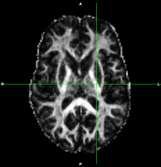
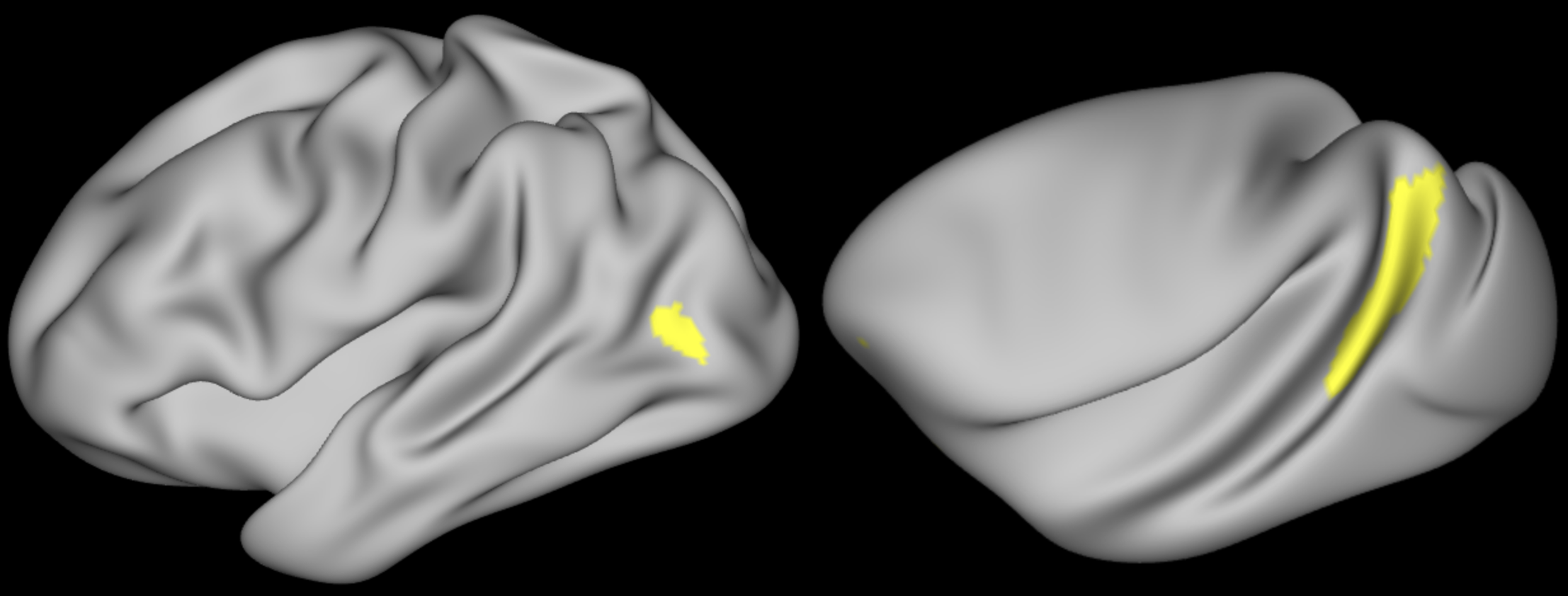
Here we will attempt to identify the tracts running through the internal capsule, which is dominated by the cortico-spinal tracts. In FSLeyes, open diffusion.bedpostX/mean_fsumsamples again. Find the co-ordinates of a voxel in the internal capsule (the white matter tract shown in the picture; running between the caudate/thalamus and the putamen/pallidum). Note down your chosen voxel location coordinates (bottom right hand side in FSLeyes).

Bring up Fdt - it should default to PROBTRACKX with single voxel as the selected seed mode.

Select diffusion.bedpostX as the Bedpostx directory and enter your selected voxel as the seed.

Choose an output name (e.g., internal_capsule), and press Go.

After the tractography has finished run ls. Note that a new directory has been created with the chosen output name. Check the contents of this directory (ls internal_capsule). One useful file is probtrackx.log, which contains the probtrackx command that was run to produce this directory. This file is useful as a reminder later on, but can also be used to, for example, run the same tractography on multiple subjects.

The main output file will be named basename_X_Y_Z.nii.gz, where basename is the same name as the directory and X, Y, and Z encode the seed voxel. This file contains for each voxel a count of how many of the streamlines intersected with that voxel. Back in FSLeyes, add this file and change the colour map to Red-Yellow. Adjust the min and max display thresholds until you get a good view of the main tract. Note the narrowness of the spatial distribution of the tractography results - this is because there is very low uncertainty in the internal capsule.

Tracking from a voxel in a non-diffusion space.

Seed points can also be specified in a space different from the native diffusion one. Here we will again run tractography from a single seed voxel, but this time using a seed defined on the subject's T1-weighted image rather than in diffusion space

Open structural/struct_brain in a new FSLeyes window and find an interesting seed location (e.g. in the corpus callosum).

In addition to the steps above (i.e., enter the input bedpostX directory, enter the seed voxel, and set an output name) we now also need to define the transformation between diffusion space and the space in which the seed is defined. In the Fdt GUI, select seed space is not diffusion. This should bring up two new fields, allowing you to specify the seed space:

• The seed-to-diff transform has already been computed for you and can be found in the structural/xfms directory (the file is called str2diff.mat).
• The Seed reference image is the image you selected the seed point from (structural/struct_brain).

Run this tractography and load the output (basename_X_Y_Z) into FSLeyes on top of the structural image (note that the output from probtrackX is always in the same space as the seed).

Tracking from voxels in MNI152 standard space

For seeds defined in standard space (e.g., from some atlas), we have an additional complication that we now need to specify a non-linear rather than linear transformation. To test this open structural/standard_brain in FSLeyes and find an interesting seed location.

You can specify a non-linear transform in the Fdt GUI by ticking the nonlinear checkbox and setting structural/xfms/standard2diff_warp and structural/xfms/diff2standard_warp as transforms and structural/standard_brain as a reference image. Note that the tractography output maps will be in standard space. How would you compute the warps to standard space if they had not already been provided for you? Answer.

Don't forget to select the bedpostX directory, enter the new seed voxel coordinates and set a name for the output directory. Then run the tractography and overlay the results on top of the standard image (with a different color map).

Seed masks are often defined in standard space rather than subject-specific space, so that the same mask can be used across many subjects. It is best practice in probtrackX to provide the transforms to standard space to probtrackX rather than the transforming the masks to diffusion space (as the latter will smooth the masks).

Using masks to impose anatomical priors

cd ~/fsl_course_data/fdt2

Here we will look at a more realistic example of tractography, where we do not seed from a single voxel, but rather from a mask. We will also use other masks to guide our tractography to reconstruct the optic radiation, which connects the lateral geniculate nucleus (LGN) of the thalamus to the primary visual cortex (V1).

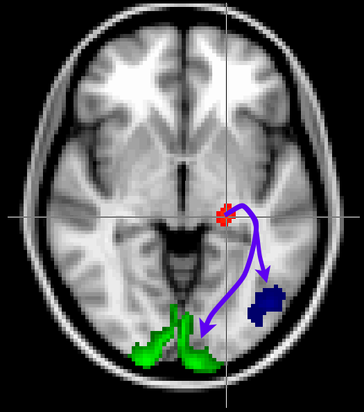
The masks have been pregenerated for you in the masks directory. Run tractography from the LGN mask (file called masks/seed_LGN_left.nii.gz). You will need to change the seed mode from single voxel to single mask. Note that this mask is in standard space, so we have to use the warp fields between standard space and diffusion space as in the example above (i.e., select Seed space is not diffusion, select nonlinear and set the appropriate transforms from the structural/xfms directory). You may want to reduce the number of samples to 500 to speed up tractography (under the Options tab). Set the output name to optic_radiation_no_waypoint and press Go.

Keep the Fdt GUI open. Now add V1 as a waypoint mask (masks/target_V1_left.nii.gz) to isolate only those tracts that reach V1. Use this V1 mask also as a termination mask to avoid tracts that reach V1 and then continue to other parts of the brain. Run tractography with these masks under the output name optic_radiation_with_waypoint.

When running from a mask the output directories contain slightly different files. The streamline density map is now called fdt_paths.nii.gz. There is now also a file called waytotal that contains the total number of valid streamlines run. This total should be much lower in the run with V1 as a waypoint mask as all the streamlines that did not reach V1 are now considered invalid.

You can check the output of both runs with:

fsleyes structural/standard_brain \
    optic_radiation_no_waypoint/fdt_paths -cm blue-lightblue \
    optic_radiation_with_waypoint/fdt_paths -cm red-yellow &

Find the optic radiation. Note that the results from the run with waypoints (in red) is much cleaner than the run without (in blue).

Rather than defining all necessary seed, waypoint, and exclusion masks yourself, you can also use XTRACT. This tool reconstructs a large number of tracts based on seed, exclusion, and waypoint masks defined in standard space. The script will also run bedpostX for you and register the diffusion data to standard space.

Estimating connectivity between brain regions

Above we recreated known white matter tracts by guiding the streamlines using masks. Here we will look at estimating the connectivity between brain matter regions by counting the number of streamlines connecting them. Whenever you work with these streamline counts keep in mind what we are actually measuring is the robustness of that connection against noise, which will be affected by confounds such as tract length or the presence of crossing fibres. Connectivity analysis will also be affected by false positive streamlines (i.e., streamlines that follow a path through the brain that does not match a true underlying tract).

Connectivity between region of interests

Here the goal is to measure the connectivity between N regions of interest. In the Fdt GUI this can be set up by:

• Set the BEDPOSTX directory to diffusion.bedpostX.
• Set Seed space to multiple masks and add any ROIs you want to include to the Masks list (you can use any masks defined in the masks directory or create your own in standard space using for example the atlases included in FSL).
• As the masks have been defined in standard space, we also need to include the transformations to standard space (i.e., check "Seed space is not diffusion", then check "nonlinear" and then set the transforms to their appropriate files in structural/xfms).
• Set the number of samples to 1 (in the Options tab) to speed up the evaluation. Running probtrackX with such a low number of streamlines can be useful for testing. For any serious analysis, we recommend using many more streamlines.
• Set the output directory name to something sensible.
• Press Go.

The output directory still contains an image fdt_paths.nii.gz which shows the path of the streamlines between the ROIs, but the main output for this analysis is the file fdt_network_matrix. Run cat on this text file to see its contents. The file contains an NxN matrix quantifying the number of streamlines between the selected ROIs that can be compared across subjects. Running such an analysis would typically require creating custom python or matlab scripts.

In this analysis we simply add up the streamlines connecting with any voxel in the region of interest. To be able to segment a region of interest, we need to consider the connectivities from individual voxels within each ROI. In the following sub-sections we will explore two ways of doing so.

Connectivity between voxels and regions of interest: hypothesis-driven segmentation

Here we will segment the thalamus based on the connectivity with the cortex. To do this we will need to estimate for every voxel in the thalamus how strongly it is connected with a number of pre-defined ROIs in the cortex.

Let's first have a look at out input masks:

fsleyes structural/standard_brain.nii.gz \
    masks/seed_thal_right.nii.gz \
    masks/cortex_*_right.nii.gz &

Ensure that all the masks have different colours, so that you can distinguish them.

seed_thal_right is the seed mask and should cover the right thalamus. From each voxel in this mask we are going to measure the number of streamlines connecting to the cortical regions, which are defined by the other masks. To run this analysis, in the Fdt GUI:

• Set the BEDPOSTX directory to diffusion.bedpostX.
• Set Seed space to single mask and set this mask to masks/seed_thal_right.
• Set the transformations between the seed mask (in standard space) and the diffusion space.
• Set the classification masks to the different cortical lobes (i.e., all the mask/cortex_*_right files).
• Set the number of samples to 10 (in the Options tab) to speed up the evaluation.
• Set the output directory name to something sensible.
• Press Go.

The objective of this type of analysis is to ask the following question: For each location in the seed mask, what is the relative probability of connection to each of my target masks? The output is therefore a single image for each target mask in which only voxels within the seed mask contain data. At each voxel within the seed mask the voxel value is the number of streamlines which reached this target mask from this seed voxel. These outputs can be found in the output directory as the seeds_to_* files. Unfortunately, 10 streamlines is not enough to get a reliable segmentation of the cortex, so we ran for you the same tractography with 2000 streamlines per voxel, which is available as the THAL2CTX_right directory.

Now overlay in FSLeyes, in turn, each of the seeds_to_* files in THAL2CTX_right. Compare the spatial distributions and probabilities of connection from different thalamic voxels to different cortical target zones. Do you see any overlap between connectivity probabilities of the different targets in the seed region? What do you think this means? Answer.

Run find_the_biggest on the outputs of seeds to targets to generate a hard segmentation of the thalamus and overlay this segmentation onto the standard brain. Something like:

find_the_biggest THAL2CTX_right/seeds_to_* biggest_segmentation

The different numbers in the output image (biggest_segmentation) each relate to a different target mask. You may want to change the colour map to something like Random.

Dense connectome between voxels: data-driven segmentation

In both cases above the connectivity from the seed region was measured based on known regions of interest. For some applications, a more precise measure of connectivity might be needed, where we consider which voxels within one ROI connect with which voxels in another ROI. If both ROIs cover the complete gray matter region the resulting matrix will contain the connectivity between each pair of gray matter voxels (i.e., a dense connectome).

In probtrackX there are three different options to generate such a connetome. Which one you need will depend on whether you want the ROIs between which you will calculate the dense connectome to also function as seed matrix (matrix1 or matrix2) or whether you want a different seed mask (matrix3):

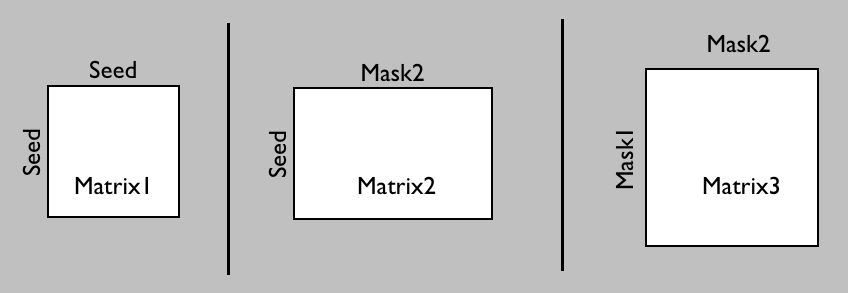
Here we will just run a simple example, which could be a first step in segmenting the thalamus in a more data-driven way than above. For this we will compute the connectivity between each voxel in the thalamus and each other voxel in the brain. In the Fdt GUI:

• Set the BEDPOSTX directory to diffusion.bedpostX
• Set Seed space to single mask and set this mask to masks/seed_thal_right
• Set the transformations between the seed mask (in standard space) and the diffusion space.
• Toggle the Matrix2 option (in the Options tab under Matrix options) and set the Tract space mask to structural/standard_brain.
• Set the number of samples to 10 (in the Options tab) to speed up the evaluation
• Set the output directory name to something sensible
• Press Go

Check the contents of the output directory using ls. A full matrix storing the connectivity between each voxel in the thalamus with each voxel in the rest of the brain would be very big, so here only a sparse representation is stored. In short, each voxel in the thalamus (i.e., the seed mask) is assigned an index, which you can look up in the coords_for_fdt_matrix2 file. Similarly, each output voxel is assigned an index, which you can look up in tract_space_coords_for_fdt_matrix2 or in the image lookup_tractspace_fdt_matrix2.nii.gz. Finally, the main output file fdt_matrix2.dot contains in each row the number of streamlines (last column) connecting a voxel in the thalamus (first column) with a voxel in the rest of the brain (second column).

This output gives us for each voxel in the thalamus the connectivity "fingerprint" with the rest of the brain. As could be seen in the lecture for the medial frontal cortex, this fingerprint can be used to segment the region by clustering these connectivity "fingerprints". This analysis would again require custom matlab or python code and is hence beyond the scope of this practical.

If you have made it through the practical so far, you have explored many of the different ways to run tractography in probtrackX. Congratulations! You can now continue with the more advanced topics below or if you prefer you can continue exploring the options above by reconstructing different white matter tracts or computing the connectivity profile of your favorite brain region.

XTRACT: automated and standardised cross-species tractography

Basics of XTRACT

XTRACT is a wrapper tool that calls probtrackX to reconstruct white matter fibre bundles. We have defined a library of tractography protocols for the human (adult and neonate) and macaque brain. Let's look at how to call XTRACT.

  xtract --help
  

As you can see, we must specify the the -bpx, -out and -species arguments. And there are many more optional arguments we may need to supply to run XTRACT. As an example, we are going to run XTRACT for the two of the superior longitudinal fasciculi (SLFs 1 and 3). First, let's look at one of the protocols we use to do this (slf1_l). Protocols are stored under $FSLDIR/data/xtract_data/. Open the protocol with a standard space brain:

    fsleyes -std1mm ${FSLDIR}/data/xtract_data/HUMAN/slf1_l/seed.nii.gz -cm green \
      ${FSLDIR}/data/xtract_data/HUMAN/slf1_l/target1.nii.gz -cm blue \
      ${FSLDIR}/data/xtract_data/HUMAN/slf1_l/target2.nii.gz -cm yellow \
      ${FSLDIR}/data/xtract_data/HUMAN/slf1_l/exclude.nii.gz -cm red &
  

The ${FSLDIR}/data/xtract_data/HUMAN/slf1_l directory contains a seed, two targets and exclusion mask used to commence and restrict tractography. The seed mask in green is a coronal ROI in the central sulcus. One of the target ROIs (yellow) is a large coronal mask in the superior parietal lobule (SPL). And the other target ROI (blue) is in the superior frontal gyrus (SFG). Exclusions are placed at the midsaggital to restrict our tract to a single hemisphere, and in the subcortex and inferior to the parietal cortex to avoid leakage to other bundles. One you've had a look at the protocol, close FSLeyes.

Running XTRACT

Let's run XTRACT to reconstruct the two bundles of the SLF (slf1_l and slf3_l). First, we can build the paths for the arguments we need to provide. We will also build a structure list file specifying the tract name and number of samples per seed voxel to use. For this practical so that XTRACT doesn't take hours on a CPU, we will use far fewer samples than normal. And because we are specifying our own structure list file, we need to tell XTRACT where to find the list and the corresponding protocol. Also note that we provide the warp fields between the native diffusion space and the standard space. These are generated using a combined FLIRT and FNIRT approach between diffusion space to standard space via the T1w space, as previously covered in the course. XTRACT uses these non-linear warp fields to transform the standard space masks to native diffusion space, where is runs tractography, and then stores results in the standard space.

    cd ~/fsl_course_data/fdt2
    mkdir ./xtract

    echo "slf1_l 0.1" > ./xtract/structureList
    echo "slf3_l 0.1" >> ./xtract/structureList

    xtract -bpx ./diffusion.bedpostX -stdwarp ./structural/xfms/standard2diff_warp \
      ./structural/xfms/diff2standard_warp -out ./xtract -species HUMAN \
      -p ${FSLDIR}/data/xtract_data/HUMAN -str ./xtract/structureList
  

Once finished, we will have a set of files for each protocol that we can visualise.

Visualising XTRACT results with xtract_viewer

xtract_viewer automatically reads the files and sets useful colourmaps and thresholds for a quick and easy visualisation of your results. xtract_viewer --help to see its usage. It's a simple tool that only requires the XTRACT results directory and what species we are working with. Run it for the SLFs we just created. It will open an FSLeyes window with the SLFs overlaid on a standard brain.

    xtract_viewer -xtract ./xtract -species HUMAN
  

Note: since we used a small number of samples, the resultant tracts will be noisy. Scroll through the slices to compare the different bundles. Try setting the images to maximum intensity projections to more easily compare the whole bundles. Close FSLeyes.

Visualising pre-baked results

The full XTRACT call takes an hour or two on a decent GPU. On CPUs, it will take many days. So, we have a pre-baked set of XTRACT results ready for you! Let's open them. Note: to avoid opening too many tracts at once, we'll specify the -tract_list argument.

    xtract_viewer -xtract ./prebaked_xtract -species HUMAN \
      -tract_list af_l,af_r,atr_l,atr_r,cbd_l,cbd_r,cst_l,cst_r,fmi,fma
  

Have a look through the tracts. We have opened the arcuate fasciculi (AF), anterior thalamic radiations (ATR), dorsal segment of the cingulum bundles (CBD), forceps major (FMA) and forceps minor (FMI). We also have a set of XTRACT tract atlases that we can visualise. Remove the tracts using the minus button, keeping the standard brain. Open the atlases tab (Settings -> Ortho View 1 -> Atlases), untick any pre-loaded atlases, scroll to the bottom of the atlases list and tick on XTRACT HCP Probabilistic Tract Atlases and click the 'Show/Hide' button. Now we can see the winner-takes-all tract atlas for 42 white matter fibre bundles. Move through the slices, place the cursor in a tract of interest and click the 'Show/Hide' button next to the tract name in the Atlases tab to show the probabilistic atlas of the tract. These show the population percent for each voxel, averaging tracts across ~1000 subjects from the Human Connectome Project (HCP). Close FSLeyes.

Simple tract-wise summary statistics with xtract_stats

One of the most common uses of white matter segmentation is to summarise tracts in terms of the microstructure and/or volume for further analysis. xtract_stats provides a quick and simple way of doing that. First, call xtract_stats for the usage:

    xtract_stats --help
  

You can see that we must specify the the XTRACT results directory -xtract, and some diffusion microstructure path -d. We can use the results from DTIFIT from the previous (fdt1) practical session. Since our XTRACT results are in standard space, we also need to specify a warp field (standard space to native space) as before. Again, we just run a subset of tracts for the sake of time. A fully pre-baked version is available here ./prebaked_xtract/prebaked_stats.csv.

    xtract_stats -xtract ./prebaked_xtract -d ../fdt1/subj1/dti_ \
      -warp ../fdt1/subj1/dti_FA ./structural/xfms/standard2diff_warp \
      -meas vol,prob,FA,MD -tract_list af_l,atr_l,cbd_l
  

Open the .csv file and have a quick look. As you can see, the tracts have been summarised in terms of their volume, probability, length and microstructural properties, ready for further analysis.

Generating connectivity fingerprints with xtract_blueprint (optional)

Connectivity fingerprints are the unique set of connections for cortical areas. We can embed the XTRACT tracts at the cortex to create cortical connectivity fingerprints, or a "connectivity blueprint". Since XTRACT is designed to provide homologous white matter fibre bundles for the human and non-human primate brain, we can do this in a way that allows us to quantitatively compare brains across species. You can build these using xtract_blueprint. This requires several inputs and is best used with surface data, so we won't run it here but we can look at the usage and results.

  xtract_blueprint --help

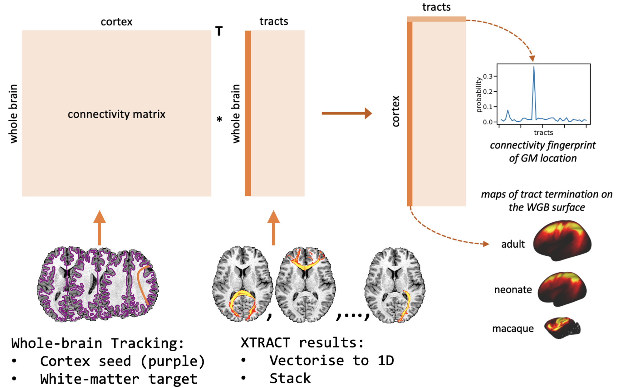
As you can see from the usage, xtract_blueprint is a two stage process. First, it runs whole-brain tractography, seeding from the cortex (the white-grey matter boundary) and targeting the whole-brain white matter, giving a cortex by WM connectivity matrix. Second, it takes the volumetric XTRACT tracts, converts them to vectors and stacks them to create a white matter by tracts matrix. These two matrices can be multiplied to give a cortex by tracts matrix, the connectivity blueprint. This image shows the process for constructing connectivity blueprints. Rows of the connectivity blueprint, cortex by tracts matrix, are connectivity fingerprints and columns are the maps of tract termination on the cortex, exampled for the neonate and adult human, and the macaque.

These are typically stored as CIFTI format files where we have a set of scalar maps representing the cortical terminations of the XTRACT tracts. For the purposes of this course, we have converted group-averaged human and macaque connectivity blueprints GIFTI metric files, so that you can view them using FSLeyes. Open the human/macaque blueprint with FSLeyes. Open the "Overlay display settings" so you can scroll through the tracts using the "Vertex data index" slider. Have a look at indices 17, 36, 38, and 40, which correspond to the frontal aslant tract (FA), and SLF bundles (adjust the display ranges to better visualise the tract maps). Visually compare them across species. Human:

  fsleyes --scene 3d ./tractography_fingerprinting/hum_L.very_inflated.resampled.surf.gii \
    --name inflated_surface --cmap brain_colours_1hot_iso \
    --vertexData ./tractography_fingerprinting/hum_aveBP.L.func.gii &

Macaque:

  fsleyes --scene 3d ./tractography_fingerprinting/mac_L.very_inflated.resampled.surf.gii \
    --name inflated_surface --cmap brain_colours_1hot_iso \
    --vertexData ./tractography_fingerprinting/mac_aveBP.L.func.gii &

Close FSLeyes. We have also recently developed xtract_divergence, which allows you to quantitatively compare these blueprints using, for example, Kullback-leibler divergence. You can compare any pair of brains, across individuals or species and create divergence maps and predictions of scalar maps. Divergence maps may be dense vertex to vertex maps giving the divergence between every vertex in brain A to every vertex in brain B, or they may be maps of divergence between ROIs and a whole-brain. Prediction of scalar maps, e.g. myelin maps, can also be performed where we use the divergence map as a warp field to transform the scalar map from brain A to brain B. Let's take a look at xtract_divergence:

  xtract_divergence --help

To example this, we will can create a divergence map between the human middle temporal (MT+) cortex and the whole of the macaque brain, which we know to be quite different across species. Our question is whether we can predict the extent of the MT+ in the macaque based on the similarity in connectivity patterns between the human and macaque brains?

  xtract_divergence -bpa ./tractography_fingerprinting/hum_aveBP.LR.dscalar.nii \
    -bpb ./tractography_fingerprinting/mac_aveBP.LR.dscalar.nii \
    -out ./tractography_fingerprinting/ \
    -masksa ./tractography_fingerprinting/hum_atlasroi.resampled.L.shape.gii ./tractography_fingerprinting/hum_atlasroi.resampled.R.shape.gii \
    -masksb ./tractography_fingerprinting/mac_atlasroi.resampled.L.shape.gii ./tractography_fingerprinting/mac_atlasroi.resampled.R.shape.gii

This creates a prediction divergence map of in the macaque brain comparing every macaque vertex to the human MT connectivity fingerprint (./tractography_fingerprinting/a_to_b_KLD.dscalar.nii). We can't open CIFTI files with FSLeyes, but can have converted it to a GIFTI so you can visualise the divergence map. Call FSLeyes:

  fsleyes --scene 3d ./tractography_fingerprinting/mac_L.very_inflated.resampled.surf.gii \
    --name "inflated_surface" --cmap brain_colours_diverging_bgy --displayRange 2.0 25.0 \
    --vertexData ./tractography_fingerprinting/mac_MT_prediction.L.func.gii &

Compare the divergence map to the actual parcellations of the human and macaue MT+ regions, shown below. You can see that the human and macaque parcels are quite different. In FSLeyes, with the selected colourmap, blue regions correspond to vertices with lower divergence to the human MT+, i.e. regions we predict to be the MT+ in the macaque. Yellow regions are highly divergent. You can see a deeper blue region in the inferior temporal sulcus. Set the max display range value to 3 to obtain a map corresponding well to the actual parcellation shown. Despite the human and macaque MT+ regions being very different, we are able to approximate the macaque MT+ based on the similarity in connectivity fingerprints between the human MT+ and macaque.

---

Making your own XTRACT protocols (optional)

Making your own protocol is simple, it's just some ROIs. Making a good protocol takes more time. Minimally, you need to specify a seed. You will also want to specify a target and exclusion mask. These can be extracted from atlas segmentations, created with e.g. fslroi, or hand-drawn masks. Typically, we construct protocols in standard space so they are generalisable across subjects. For the human brain, we use the MNI152 space. Have a go. Build a protocol to reconstruct a tract of interest. All ROIs must be placed under a single directory e.g. ./protdir/my_tract. The seed must be called "seed.nii.gz", the target "target.nii.gz" and the exclusion "exclude.nii.gz". You can have multiple targets ("target1.nii.gz", "target2.nii.gz", etc...). You can also specify that the streamline must pass through the targets in numerical order using a empty text file called "wayorder" in the tract protocol directory. Likewise, with a file called "invert", you can specify an inverted run where the seed and final target reverse roles and the final tract is the sum of the two runs. As well as the protocol, you need to specify a structure list file like we did earlier. Each line should contain two columns specifying the tract name (as it appears in the directory name, e.g. my_tract) and the number of samples per seed in thousands, e.g. "my_tract 5" You can then call XTRACT specify the path of your protocol:

  xtract -bpx ./diffusion.bedpostX \
    -stdwarp ./structural/xfms/standard2diff_warp ./structural/xfms/diff2standard_warp \
    -out ./xtract -species HUMAN -p ./protdir/my_tract -str ./protdir/structureList

---

Bedpostx model specification (optional)

cd ~/fsl_course_data/fdt2

In this section we will see how the choice of the bedpostx model can affect the fitting results.

We will compare model 1 (ball & sticks, single diffusion coefficient) to model 2 (ball and sticks, continuous gamma distribution of diffusion coefficients) on our multi-shell data.

Model 2 should be better suited to deal with multi-shell data, as the apparent diffusion coefficient can change with the b-value. Using model 2 tends to reduce overfitting (i.e., spurious fibre orientations).

Open FSLeyes by typing the following command in your terminal:

fsleyes \
  diffusion.bedpostX/mean_fsumsamples.nii.gz -or 0 0.8 \
  diffusion_model1.bedpostX/mean_f2samples.nii.gz \
    -cm blue-lightblue -or 0.05 0.2 \
  diffusion.bedpostX/mean_f2samples.nii.gz \
    -cm red-yellow -or 0.05 0.2 \
  diffusion_model1.bedpostX/dyads1.nii.gz \
    -ot linevector -xc 0 0 0 -yc 0 0 0 -zc 0 0 0 -lw 2 \
  diffusion_model1.bedpostX/dyads2_thr0.05.nii.gz \
    -ot linevector -xc 1 1 1 -yc 1 1 1 -zc 1 1 1 -lw 2 &

This loads the fitted orientations using model 1 (single diffusion coefficient), as well as the volume fractions of the secondary fibre orientation for both models 1 and 2.

First, deselect the dyads files, and examine the volume fractions (mean_f2samples). Model 1 should be displayed in Blue and model 2 in Red-Yellow.

The first thing that is immediately visible is that many more voxels survive a 0.05 thresholding on the volume fractions of the secondary fibre when using model 1. This is particularly true at interfaces between grey/white/CSF tissues, where partial volume is likely to occur, and it indicates that the model is overfitting the data.

Now examine the dyads in the voxels where a secondary fibre is estimated when using model 1 but not model 2 (i.e., the blue voxels). You can observe that in most of them, especially in those closer to tissue boundaries (grey/white/CSF interface) the second dyad is perpendicular to the first one, but does not show spatial continuity when compared to neighbouring dyads.

Partial volume effects can cause the signal to decay non mono-exponentially when increasing the b-value. Since model 1 has a single diffusion coefficient, it can only capture this feature of the data by adding a perpendicular second dyad, which fits the data better but does not correspond to a genuine (anatomical) fibre orientation.

---

Using surfaces to constrain tractography (optional)

cd ~/fsl_course_data/fdt2/surfaces

All previous examples use volumetric seeds and constraint masks. Probtrackx2 also supports surface files (e.g., generated using FreeSurfer or Caret).

In this example use of surfaces, we consider the case where FreeSurfer has been used to generate a cortical surface, and show how such surface can be used in probtrackx2.

In the current folder you will find the high-resolution T1-weighted volume produced by the FreeSurfer recon-all command (orig.nii.gz), the necessary transformation matrices to go from FreeSurfer anatomical space to diffusion space and the white/grey matter boundary surfaces for the left (lh.cortex.gii) and right (rh.cortex.gii) hemispheres. For details on how to generate these files, see the relevant documentation.

Here, we will see an example where, in order to avoid spurious connections that connect adjacent gyri, we impose the convoluted WM/GM boundary surface as a termination mask. Tracking will be performed again in anatomical space as defined by the orig.nii.gz volume. We will first run an example without any surface constraints from a seed close to the cortex.

The command:

echo "97 96 125" > svox.txt

creates a text file called svox.txt that contains the string 97 96 125. This could also be created using your preferred "plain" text editor.

In your terminal type:

echo "97 96 125" > svox.txt
probtrackx2 \
  --samples=../diffusion.bedpostX/merged \
  --mask=../diffusion.bedpostX/nodif_brain_mask.nii.gz \
  -x svox.txt \
  --xfm=freesurfer2fa.mat --seedref=orig.nii.gz \
  --loopcheck --simple --forcedir \
  --opd -V 1 --dir=Tracts --out=no_surf

The next commands will include as termination masks the wm/gm boundaries of both hemispheres:

echo lh.cortex.gii > stop.txt
echo rh.cortex.gii >> stop.txt
probtrackx2 \
  --samples=../diffusion.bedpostX/merged \
  --mask=../diffusion.bedpostX/nodif_brain_mask.nii.gz \
  -x svox.txt \
  --xfm=freesurfer2fa.mat --seedref=orig.nii.gz \
  --loopcheck --simple --forcedir --opd -V 1 \
  --dir=Tracts --out=surf --meshspace=freesurfer --stop=stop.txt

After the results have been computed, open FSLeyes with the following command:

fsleyes -ds world \
  orig.nii.gz rh.cort.nii.gz -cm green \
  lh.cort.nii.gz -cm copper \
  Tracts/no_surf_97_96_125 -cm blue-lightblue -or 10 1000 \
  Tracts/surf_97_96_125 -cm red-yellow -or 10 1000

This loads the tractography results overlaid on top of the high-resolution anatomical volume together with the surface boundaries. The results obtained when using the surfaces as termination masks should be displayed in red-yellow and those obtained without surface contraints should be in blue-lightblue.

Go to slice Y=91. Observe how, when surfaces are not used as termination masks, the tracts in blue wrongly connect two adjacent gyri by passing through a sulcus.

---

The End.