Fitting MEGA-edited Spectroscopy Data
This mini practical covers Mega-edited spectroscopy fitting as introduced in Chapter 4. As with all these mini-practicals, instructions on how to run FSL commands can be found on the Getting Started page.
Please download the dataset for this example here:
Data download
Once it is downloaded, move it to your preferred working directory and unzip it there.
unzip data_ch4_mega.zip
cd  data_ch4_mega
Looking at the data
We begin by looking at the MEGA data. There are two datasets, with the editing pulses either turned ON or OFF. Let us look at the data in FSLeyes.
cd processed
fsleyes edit_0 edit_1 &
Toggle the edit_1 data on and off to see the difference. You can also load the difference data diff.nii.gz.
You should see that the GABA peaks are nice and prominent in the difference spectrum. We will fit the model
to this difference spectrum. But first, we need to create basis spectra.
Basis spectra
You should be able to see two sequence descriptions for the ON and OFF experiment (called MEGAPRESS_ON.json and MEGAPRESS_OFF.json.
Let's use these to simulate metabolite bases (this may take a while, so if you can't wait you should be able to find pre-calculated bases in the basis folder).
fsl_mrs_sim -b metab.txt -p -2 -o basis_off MEGAPRESS_OFF.json
fsl_mrs_sim -b metab.txt -p -2 -o basis_on MEGAPRESS_ON.json
Visualise the ON and OFF basis spectra with mrs_tools vis. What do you notice?
Let's take the difference so we can use it as a basis for our fitting:
basis_tools diff --add_or_sub sub basis_on basis_off basis_diff
Look at the diffence basis:
basis_tools vis basis_diff
You should be able to see that many of the metabolites have a flat spectrum. This is because they were not affected by the editing pulse. As they won't have any effect on the fitting, we can exclude them from the basis set. Let's create a new, simplified basis set folder:
mkdir basis_diff_reduced
cp basis_diff/{GABA,Gln,Glu,GSH,NAA,NAAG}.json basis_diff_reduced
Before we run the fitting, one last thing we need to do is to include a basis for macromolecules. This is a bit complicated
and still an area of research, but a proxy for a macromolecule difference spectrum is a couple of broadened peaks around 0.9ppm and 3ppm with
a ratio of 3:2. We will create a MM basis set from a short JSON description of this as if it was a spin system. Copy the following into a text file and call it MM.json.
{"MM":[
    {"j": [[]], "shifts":[0.917,0.915,0.913], "name": "MM09","scaleFactor": 1},
    {"j": [[]], "shifts":[3.03,3.03],         "name": "MM30","scaleFactor": 1}
    ]
}
Now we can simulate a basis with the edit-OFF sequence (if it asks to overwrite, choose No)
fsl_mrs_sim -s MM.json -p -2 MEGAPRESS_OFF.json
Now the MM.json file has been changed to represent a MM basis. Move it to the basis folder and visualise:
mv MM.json basis_diff_reduced
mrs_tools vis basis_diff_reduced
Good, we are ready to do some fitting.
Fitting edited spectra
Fitting edited spectra is done in almost exactly the same way as fitting normal spectra, as long as we have created the difference spectrum and a corresponding basis.
The only differences are:
- We need to use a different internal reference to Creatine, as we have removed Creatine from the basis (it is not present in the difference spectrum). We use NAA instead.
- We combine GABA and MM to get GABA+.
- We also combine Glu, Gln, and GSH on the one hand, and NAA and NAAG on the other due to their high correlation.
In the processed folder, you should be able to find the difference spectrum as a NIFTI file. Run the command
below to do the fitting:
fsl_mrs --data processed/diff.nii.gz \
        --basis basis_diff_reduced \
        --output fit \
        --baseline spline,stiff \
        --metab_groups MM \
        --combine Glu Gln GSH --combine GABA MM --combine NAA NAAG \
        --internal_ref NAA \
        --report
This should be quick to run. Open the HTML report and examine the results.
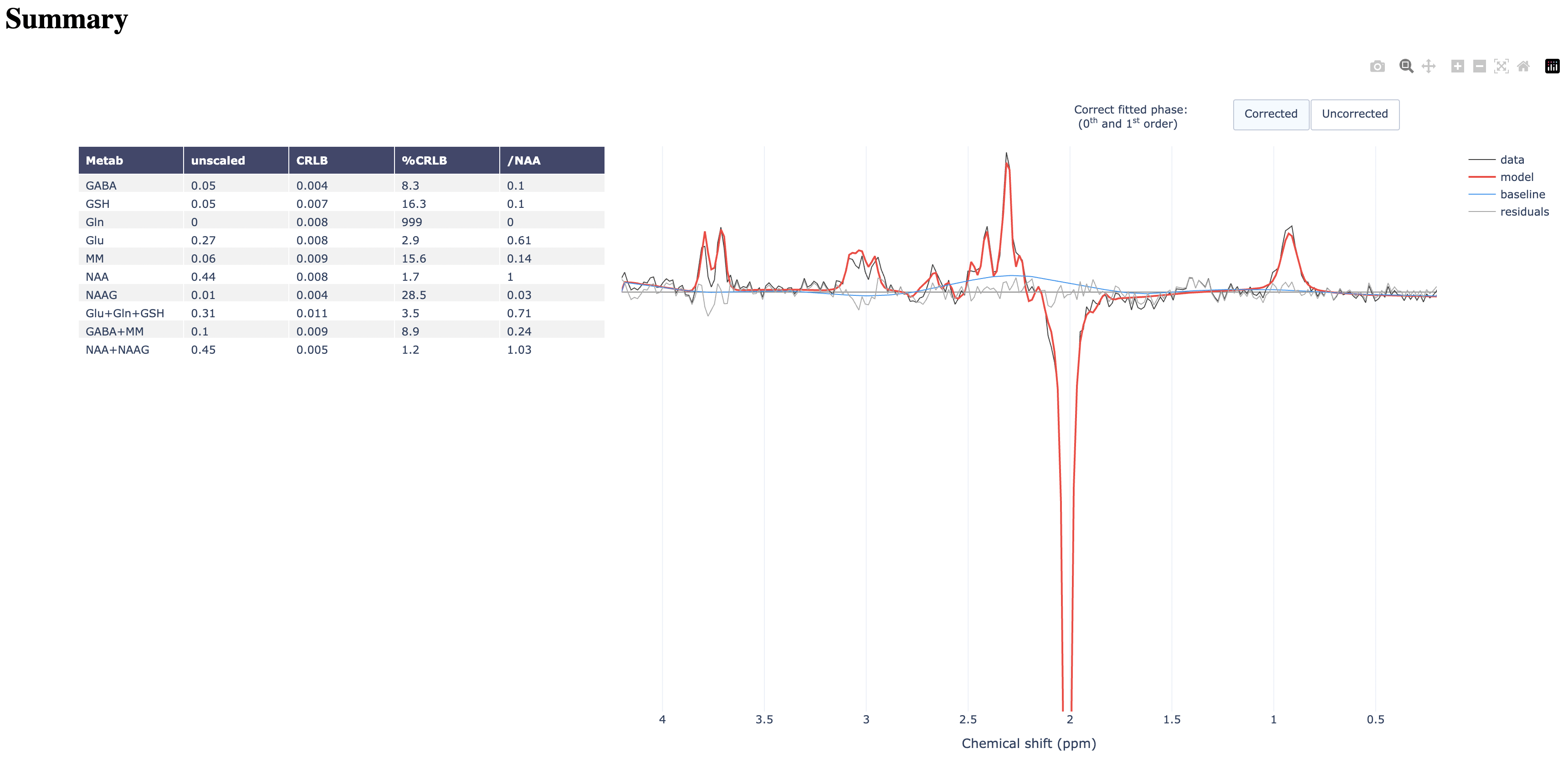
The End!