Basis Simulation

This mini practical covers the following example box in Chapter 4: "Simulating a basis". The box appears on Page 105.
As with all these mini-practicals, instructions on how to run FSL commands can be found on the Getting Started page.

Please download the dataset for this example here:

Data download

Once it is downloaded, move it to your preferred working directory and unzip it there.

unzip data_ch4_basis.zip
cd  data_ch4_basis

---

Simulating basis spectra typically requires three steps:

Sequence description

Creating a JSON text file that describes the MRS sequence.

Simulation

Running the FSL-MRS basis simulator.

Macromolecules

Adding a macromolecule spectrum to the basis.

Sequence description

To create high-quality basis spectra, the simulator must be provided with an accurate description of the MRS sequence. The description contains:

• the radio-frequency (RF) pulses,
• the slice selection and rephase gradients,
• time delays between pulses,
• information about the voxel size,
• scanner hardware and acquisition information.

All of this is contained in a simply formatted and human-readable JSON file. An example sequence description is packaged with the practical. We will go through it section by section to illustrate how it was created.

cd basis_creation
cat steam.json

The JSON file contains the following important fields that we will tackle in turn. For a full reference see the online documentation.

• RF, delays, & rephaseAreas
• CoherenceFilter
• Spatial resolution parameters (x, y, z, resolution)
• B0 & centralShift
• Rx_* parameters
• Other parameters

The STEAM sequence

To understand this file, first we must understand the structure of the STEAM sequence. For reference in this process we have included a schematic STEAM sequence diagram.

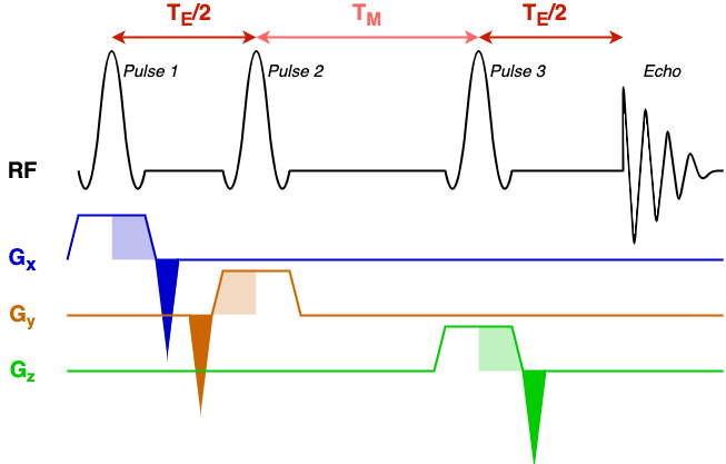
The diagram has a black line denoting RF events (RF pulses and the echo that is formed), and three coloured gradient axes: x, y, and z. In this simple sequence the same 90-degree pulse is repeated three times to form a 'stimulated' echo. Each pulse has an associated slice select gradient, one for each axis, all with the same gradient strength (the voxel has equal dimensions in x, y, and z). Before, or after, the slice-select gradient is a rephasing gradient (dark shaded area) with area equal to half the slice select gradient (light shaded area).

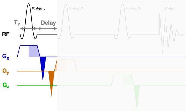
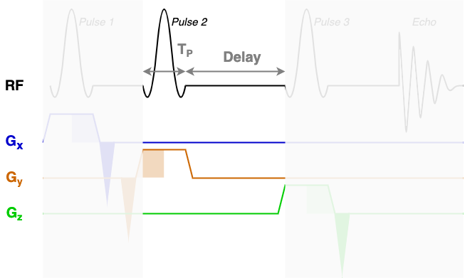
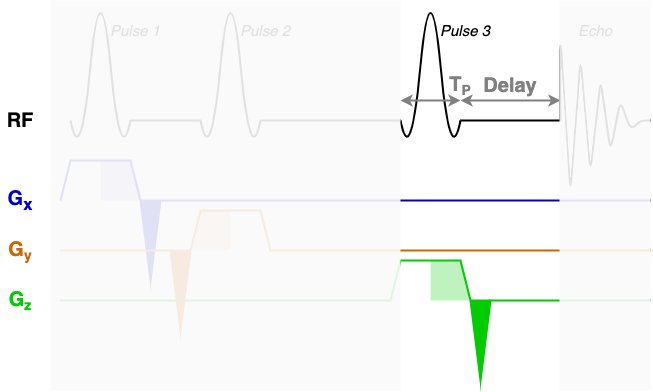
Sequence blocks

At the core of the sequence description format, an MRS sequence is split up into blocks containing a single RF pulse, associated gradients, and a time delay. The next three diagrams show each of the three sequence blocks in this STEAM sequence. In the sequence description we will describe the RF and gradients in each of the highlighted areas.

RF, delays, & rephaseAreas

Three fields define the majority of the sequence information in the JSON file. These are RF, delays, & rephaseAreas. Try inspecting the packaged sequence description file in a text editor. Take a look at each of those parameters and what data they contain.

You will find that RF contains three blocks of almost identical information. Each block encodes one of the three RF pulses (Pulse 1, Pulse 2, and Pulse 3) using the following fields:

• amp: The pulse amplitude modulation as a list. Typically in units of hertz - a 1 ms hard 90-degree pulse would have an amplitude of 250 Hz.
• phase: The pulse phase modulation as a list. In radians.
• time: The total duration of the pulse (T_P in the diagrams above). In seconds.
• grad: The slice selection gradient. This is the only field that changes between the blocks, with the constant slice selection gradient iterated over the x, y, and z axes (first, second, and third elements). In "GradUnit"/m, where you can specify "GradUnit" in the JSON file (typically mT).
• frequencyOffset: The frequency offset of the pulse, referenced from the central frequency (see centralShift). In this data the value of -580 MHz corresponds to a shift of -1.95 ppm to centre the pulse in the middle of the spectrum around 2.7ppm. The frequency offset is calculated as frequencyOffset[MHz] = (target[ppm]-centralShift[ppm])*B0[tesla]*GyromagneticRatio[MHz/tesla]
• phaseOffset: Fixed phase offset for the pulse, typically 0. In radians.

The delays field is a list with a single delay value per block. In this sequence we have three blocks with three delay times as marked in the figures above.

The rephaseAreas field is a 3 (x, y, z) by N_blocks array. This array encodes the areas of the rephase gradients. During the first block there are two rephase gradients of equal area on the x and y axes([-5.145e-03, -5.145e-03, 0.000e+00]), in the second block there are no rephase areas ([ 0.000e+00, 0.000e+00, 0.000e+00]), in the third block there is a single rephase gradient on the z axis ([ 0.000e+00, 0.000e+00, -5.145e-03]). Note that the areas are negative as the slice selection gradients all have positive magnitude.

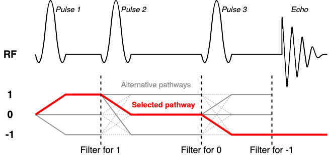
CoherenceFilter

Typically as SVS sequences are repeated to build up temporal averages a series of 'spoiler' gradients are changed incrementally to ensure that unwanted coherence pathways are prevented from appearing in the final averaged spectrum (for example due to imperfect pulses). To copy this approach in simulation would require multiple (tens of) repeated simulations to be run, each with complex gradient structure. Instead FSL-MRS implements a coherence filter to select only the desired coherence pathway.

A discussion of coherence pathways goes beyond this practical, but in brief we want to select a single sequence-dependent pathway from the many that are generated by multiple RF pulses. For STEAM and spin-1/2 systems this corresponds to the [1, 0, -1] pathway. An excellent resource for this is Landheer & Juchem's work. For this, and all other, STEAM sequences we set the coherenceFilter field to [1, 0, -1]. This means that after each RF pulse and delay only the coherence in the filter is allowed to proceed.

Spatial resolution parameters (x, y, z, resolution)

For accurate basis spectra, the simulation must be carried out over a fine grid of spatial points, before summation in a final step. We therefore tell the simulation over what spatial grid to simulate. A good recommendation is to set the grid in each dimension (x, y, & z) to twice the voxel size. Here the voxel size was 25 mm isotropic, thefore we set each field to [-25,25] so that simulations take place 25 mm around the centre in each direction (50 mm in total).

The resolution parameter then sets how coarse or fine the grid is for simulation. Always start with a coarse grid (e.g. 5-10) for debugging and tests, as this will speed up the process. A final simulation should be carried out with many points in each direction; in the 40-60 point range.

B0 & centralShift

The B0 parameter sets the main magnetic field strength, which should match the field strength of your scanner. Note that many scanners are not quite the field strength advertised. A 3 tesla scanner might actually be 2.89 T, or a 7 tesla 6.98 T. This information can be found by inspecting the data which the simulation is being carried out for i.e. by running mrs_tools info on the raw data.

The centralShift parameter indicates where the central frequency of the scanner was set during any acquisition. Typically, for proton MRS this would be set to the water frequency. Hence to reference between the chemical shift scale - with a somewhat arbitrary zero reference - and the one used experimentally we set this parameter to the chemical shift of water: 4.65 ppm.

Rx_* parameters

There are four parameters which are used to control the appearance of the simulated basis spectra. These are as follows:

• Rx_Points: This controls how many time points will be recorded from the echo in the simulation.
• Rx_SW: This controls the simulated receiver bandwidth (AKA sweep width).
• Rx_LW: The amount of lorentzian broadening applied to the simulated peaks. Should be low (1-2 Hz).
• Rx_Phase: An optional parameter that controls the output phase of the signal. This can be provided automatically by the simulator (see below).

The total simulated time (Rx_Points * 1/Rx_SW) should be high, so that the spectra can be interpolated down to the actual acquisition parameters. Here we have set Rx_SW to 6000 Hz and Rx_Points to 8192 for a total simulated time of 1.37 s.

Other parameters

Some of the remaining parameters, sequenceName and description, allow free form text description of the sequence being simulated.

The units parameters: RFUnits, GradUnits, and spaceUnits, allow the user to specify what units some of the parameters are defined in. See the online documentation for more information.

Open up the provided sequence description in an editor and turn down the simulation resolution from [30, 30, 30] to [5, 5, 5]. This should make the next step faster, but more inaccurate; fine for this demo.

---

Simulation

Compared to the previous section running the simulator is simple. The simulator is called using fsl_mrs_sim. The user must supply the sequence description and a list of metabolites (or custom described spin systems) to the simulator. The simulator knows about a predefined list of metabolites, meaning the user can just specify their name.

fsl_mrs_sim -b metabs.txt -p -2.0 -o my_steam_basis steam.json

In addition to a text list of metabolites supplied in metabs.txt we have added a -p -2.0 flag and -o my_steam_basis. The first automatically phases the spectra (which otherwise would have arbitrary phase) using a peak at -2.0 ppm from the central shift (I.e. 4.65 - 2.0 = 2.65 ppm). The second -o specifies an output location. Try looking at the created basis spectrum, using mrs_tools vis.

mrs_tools vis my_steam_basis/

Now let us compare the basis under different settings. First, we will look at the effect of the simulation grid. We will then look at what happens for different echo times.

Create a copy of the JSON file but change the grid resolution to 40x40x40. Save it under a different name (e.g. steam_40res.json). To save time, we will only simulate a few metabolites (using the -m option instead of -b):

fsl_mrs_sim -m Glu,Lac -p -2.0 -o my_steam_basis steam.json
fsl_mrs_sim -m Glu,Lac -p -2.0 -o my_steam_basis_40res steam_40res.json

Compare the two results using mri_tools vis.

Now create another JSON file but this time with a longer echo time. Looking at the sequence diagram at the top, you should be able to see that the echo time is composed of the first and last delays, plus half of the first pulse duration, half of the second, and the full duration of the third pulse, adding up to TE=11ms. Let's make this a 50ms echo time by increasing the first and last delays by the same amount ((50-11)/2=19.5ms=0.0195s). Save the result in a file called steam_TE50.json.

fsl_mrs_sim -m Glu,Lac -p -2.0 -o my_steam_basis_50ms steam_50ms.json

Compare the two results using mri_tools vis.

---

Macromolecules

Macromolecular basis sets are typically created by empirical measurement of metabolite-nulled spectra. The spectra should be measured using a very similar sequence to the target sequence, in a similar population to the study population, and from a similar anatomical region. The full process is beyond the scope of this practical. However, fsl_mrs_sim can be easily made to incorporate a pre-measured macromolecule basis into one that it is simulating.

Re-run the above command but add -MM MM.json. MM.json contains a single MM basis spectrum.

fsl_mrs_sim -b metabs.txt -p -2.0 --MM MM.json -o my_steam_basis_with_mm steam.json

Once again look at the result using mrs_tools vis. The basis set should now contain a MM spectrum.

If you don't have access to a measured MM spectrum, you can use the default one in FSL_MRS, which consists of several broad peaks at specific frequencies and with predefined relative amplitudes

To do this, you can first use the simulator to create your basis, then use basis_tools add_set to add a MM basis file to your basis folder:

fsl_mrs_sim -b metabs.txt -p -2.0 -o my_steam_basis steam.json
basis_tools add_set --add_MM my_steam_basis my_steam_basis_withMM

Look at the new basis and try to identify the new MM spectrum. Compare that with the measured MM spectrum (MM.json). You should be able to see that the default MM consists of separate peaks.

---

The End!