Visualising your data

This mini practical covers two example boxes in Chapter 3: "Visualisation" on page 78, and "Apodization" on page 79. As with all these mini-practicals, instructions on how to run FSL commands can be found on the Getting Started page.

Please download the dataset for this example using the button below. After download unzip the contents into a directory called data_ch3_vis.

Data download

FSL-MRS has a number of tools that can help you view your data and inspect the results of processing and fitting. This practical will take you through some of key ones. You'll see others generated during the processing and fitting stages in the later practicals. We will also see how to use a quick processing tool to reduce the visual impact of noise.

Example Box: Visualisation

FSL-MRS has a quick command line tool for viewing NIfTI-MRS files mrs_tools vis and also integrates with FSL's amazing image viewer FSLeyes.

mrs_tools vis

mrs_tools vis is a command-line tool for viewing NIfTI-MRS files. Try running it on the example unedited data data_ch3_vis/unedited.nii.gz.

mrs_tools vis data_ch3_vis/unedited.nii.gz

The tool will perform very basic processing, including a data-driven coil combination to present you with a recognisable single spectrum.

Clearly not all processing steps have been applied (for that, see the next practical), and the spectrum isn't optimal, but it is sufficient to understand the data. Now try running on the packaged water reference.

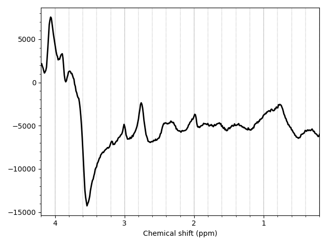
mrs_tools vis data_ch3_vis/wref.nii.gz

The result looks a bit odd. You are mostly seeing eddy current induced side bands on the water peak, mixed in with metabolite signal.

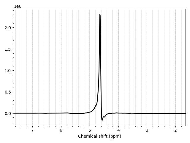
Now Use the --ppmlim argument to display the full data range.

mrs_tools vis --ppmlim 1.65 7.65 data_ch3_vis/wref.nii.gz

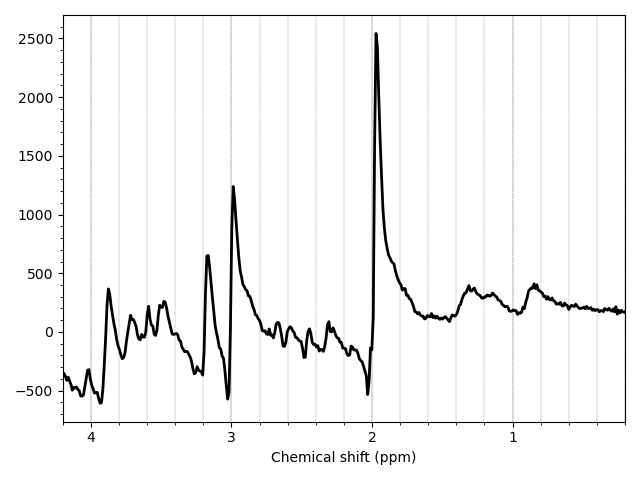
Sometimes, it might be useful to see the data where the original dimensionality hasn't been removed: averaged, coil-combined, differenced, etc. To achieve this use the --display_dim combined with the appropriate dimension tag (see the previous practical on data handling). For example, try to figure out the command to achieve this with the packaged edited data edited.nii.gz in order to display the two entries in the DIM_EDIT dimension. Click here to reveal the command.

mrs_tools vis --display_dim DIM_EDIT data_ch3_vis/edited.nii.gz

This still has an additional "mean" spectrum plotted, useful for the temporal averages dimension, DIM_DYN, but less useful here. You can suppress this by specifying --no_mean as an additional argument. The final result should look like the following image.

mrs_view and MRSI

mrs_tools vis can be used to view MRSI data, and can accept a --mask argument which selects voxels to view based on a binary NIfTI image. However, execution is slow and clunky for 3D data.

We strongly recommend using FSLeyes for visualising MRSI data.

FSLeyes

FSLeyes is FSL's dedicated image viewer. FSL-MRS extends FSL to work with MRS(I) data, allowing you to view your spectroscopic data next to and overlaid on imaging data. Load some spectroscopic data (and associated T1 structural image) into FSLeyes' MRS interface by specifying the -smrs option.

fsleyes -smrs data_ch3_vis/T1_biascorr.nii.gz  data_ch3_vis/unedited_processed.nii.gz

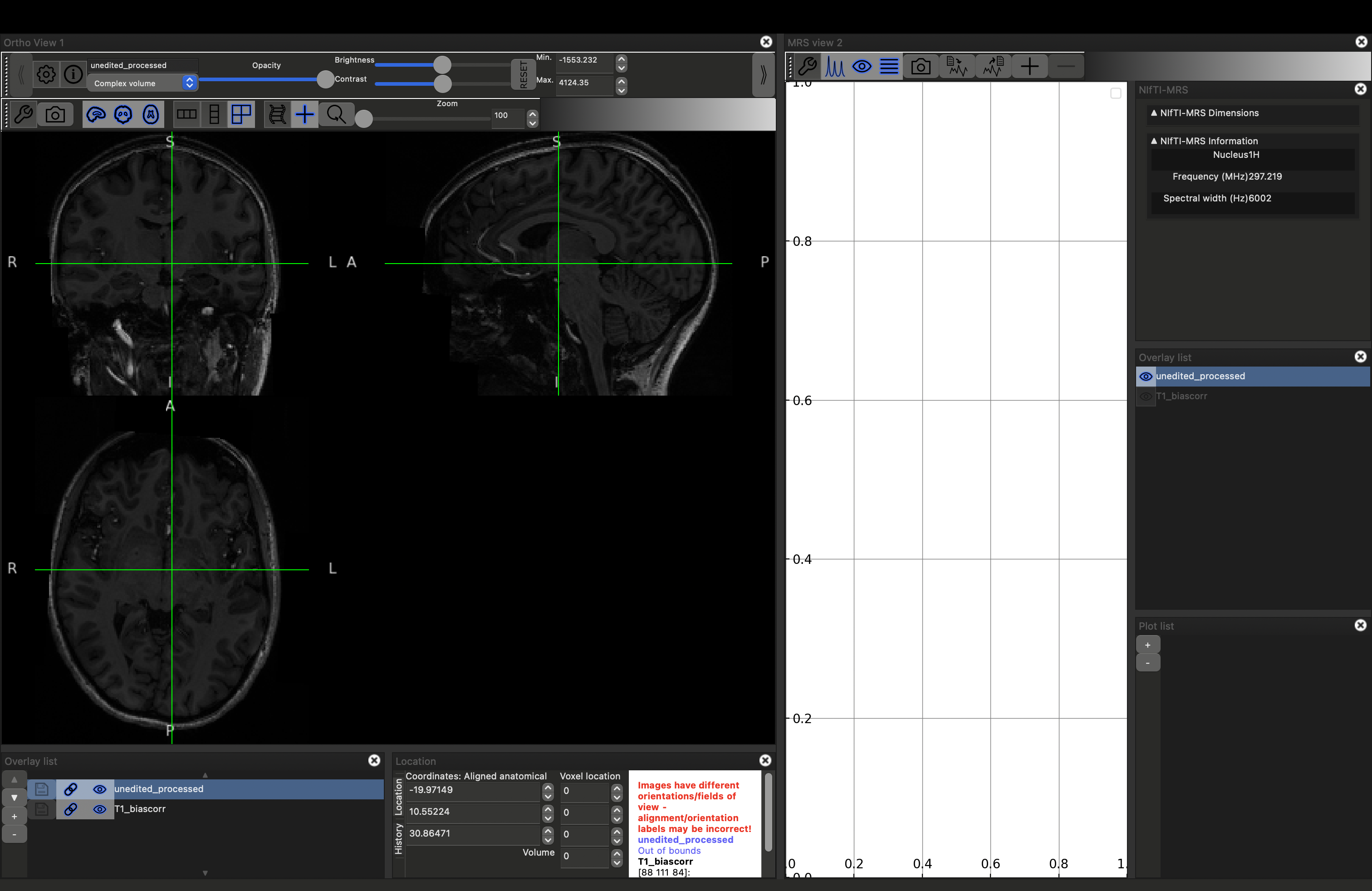
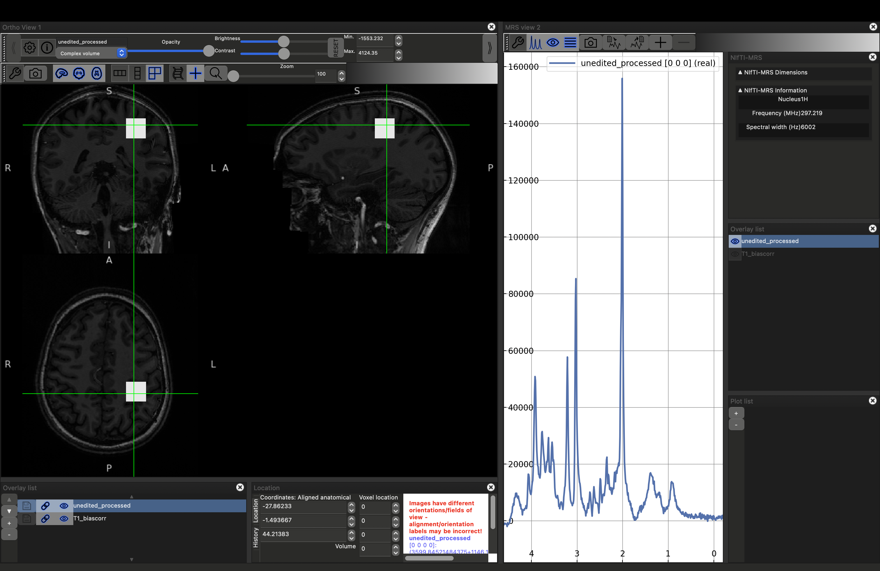
This will load the data and the MRS viewer. The MRS data will only appear if the green cross-hairs are over the voxel. Scroll to a more superior position to see the SVS voxel position. Place the cursor over it (and click), you should see the spectrum appear on the right.

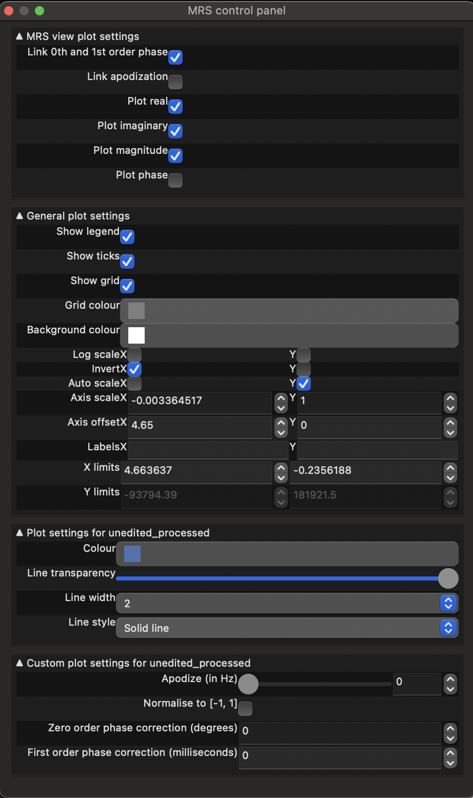
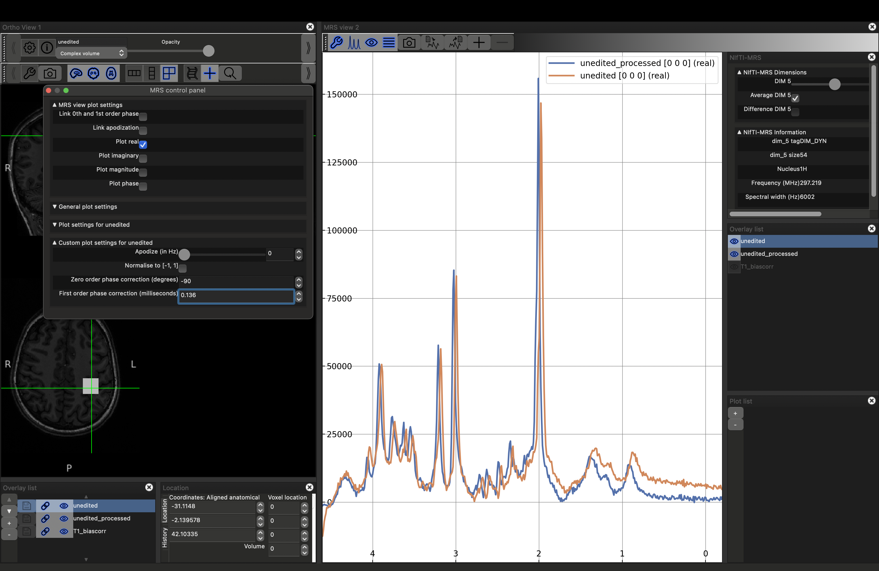
You can visualise the different projections: real (default), imaginary and magnitude, by opening the MRS control panel (click the spanner button above the spectrum). Select the projection by checking the Plot {real|imaginary|magnitude|phase} options.

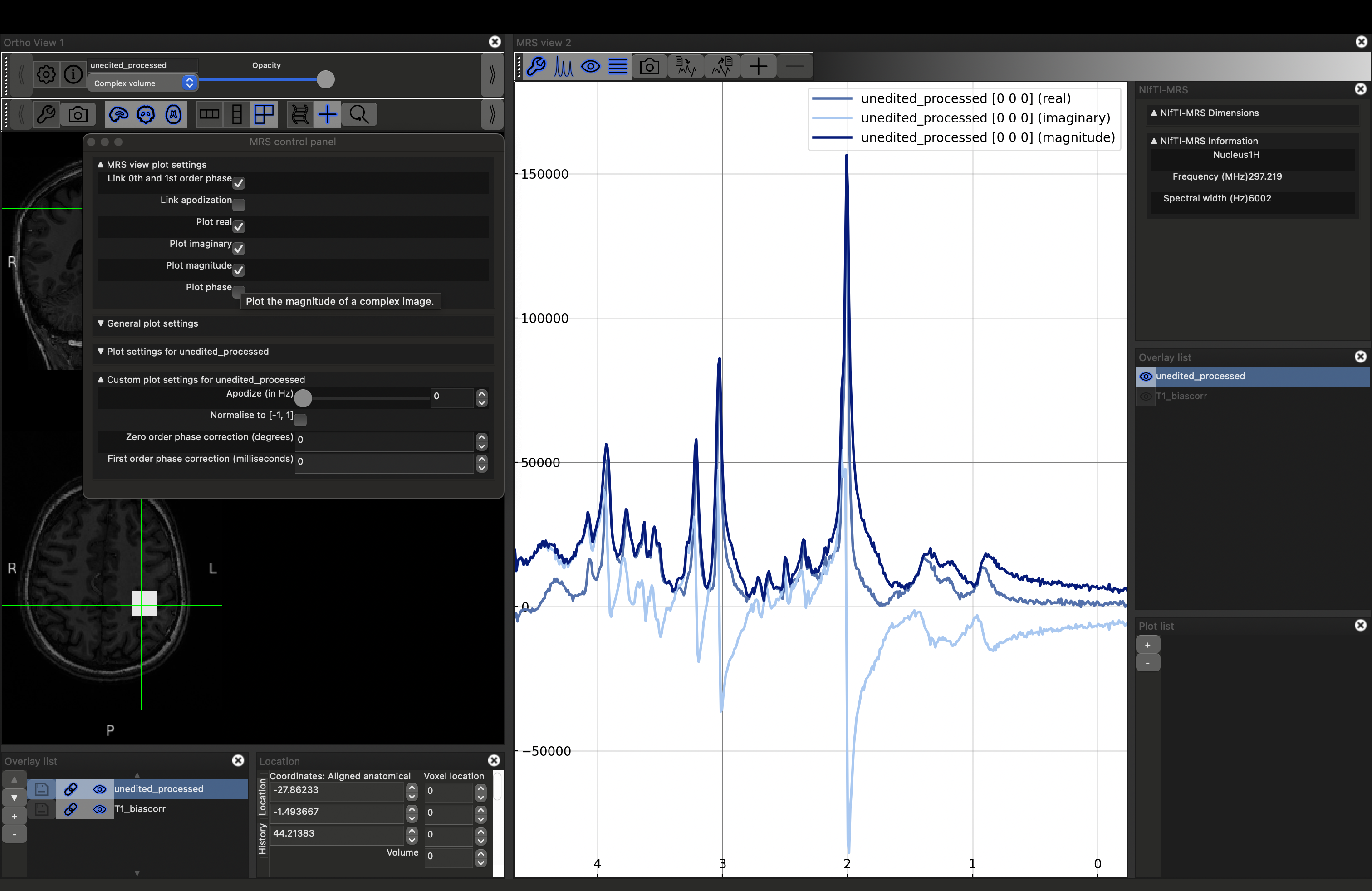
More options for controlling the appearance of the plot can be accessed by expanding other sections in the control panel.

You can also adjust the appearance of the spectrum using:

• left-click and drag to pan,
• right-click and drag to zoom,
• shift + left-click and drag to set zero-order phase, and
• ctrl + left-click and drag to set first-order phase.

FSLeyes with multi-dimensional data

Under the File menu, use the Add from file option to add the data_ch3_vis/unedited.nii.gz file. Nothing will change in the left hand view (this is the same data, before processing, so voxels overlap), but a second, noisier appearing spectrum will appear in the right-hand panel.

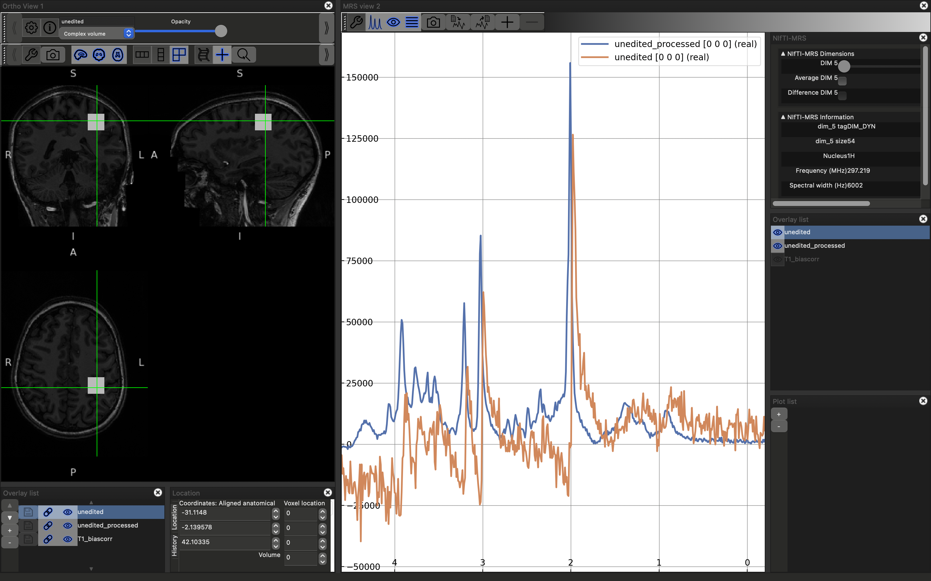
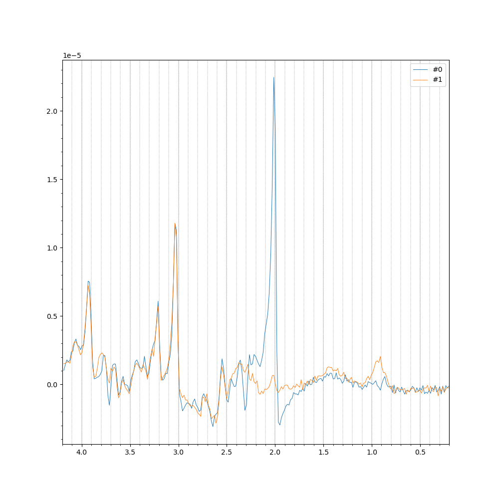
Note that there is now a slider visible in the upper right NIfTI-MRS panel. Try moving this slider, it will display each of the 54 temporal averages, acquired one per TR, in turn. Now try checking the "Average DIM 5" option.

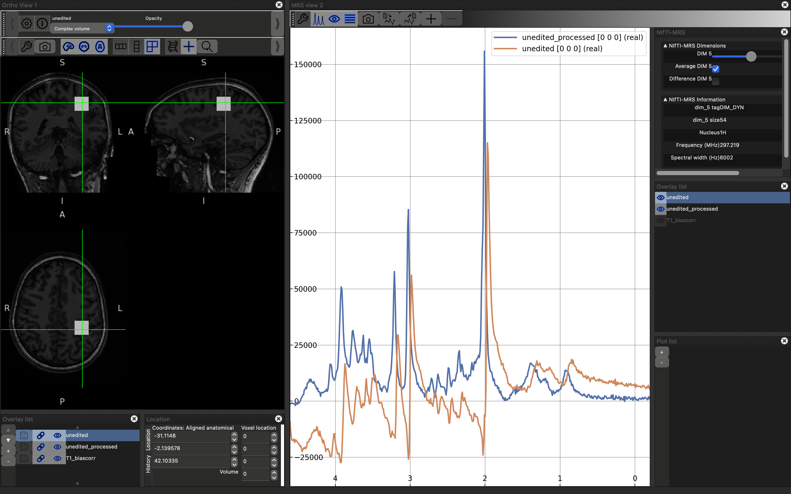
You will now see the spectrum is roughly the same quality as the processed version. However there is some phase (both zero and first order) present in the unprocessed case. If you try to apply phase using the click and drag options described above both spectra will change together. Instead reopen the control panel and deselect Link 0th and 1st order phase, then, with unedited highlighted in the right-hand Overlay list, use the phase controls at the bottom fo the control panel to make the spectra look as similar as possible. Click here to reveal the results.

Answer: zero-order = -90 degrees, first-order = 0.136 ms (equivalent to slightly less than one dwell time point.)

Note that the two spectra aren't identical even after phasing, as other processing steps, e.g. frequency alignment and eddy current correction, haven't been applied.

FSLeyes for fitting and results

We will revisit FSLeyes later, to see how you can use it for viewing MRSI fitting results, in the Chapter 4 Example Box: Fitting.

Other tools: HTML reports and fsl_mrs_summarise

FSL-MRS's processing and fitting tools create interactive HTML reports to help users assess the quality of each stage. You will find out about these later, but for now you can get a impression of a report by running:

firefox data_ch3_vis/fitting_report.html

You will also see FSL-MRS's cross-subject summary dashboard tool fsl_mrs_summarise in the Chapter 4 practical "MRS Fitting Visualisation".

Example Box: Apodization

Apodization refers to a processing step that applies a filter to the time domain FID signal, typically to increase SNR. It achieves this by down-weighting the predominantly noise-containing points at the end of the FID, whilst smoothly preserving the points at the start of the FID.

Note: A filter should only be used as a visualisation aid, and should not be used prior to other processing or fitting steps. The filter changes the noise statistics of the signal, invalidating assumptions used later.

Investigate the effect of apodization on a noisy signal. Load the unprocessed data into FSLeyes, open the control panel in the MRS View (click the spanner in the right hand view), and move the Apodize (in Hz) slider. What happens?

fsleyes -smrs data_ch3_vis/unedited.nii.gz 

The most common apodization filter used is a decaying exponential, which is a matched filter if we assume purely lorentzian line shapes. For any peak, we can achieve maximum SNR by applying an exponential filter with a width equal to the full-width-at-half-maximum of the peak. Note, that therefore, different peaks, even those arising from the same metabolite, may achieve optimum SNR at different filter widths.

In addition to the interactive apodisation shown above, we can apply an equivalent filter using FSL-MRS's command line tools. Contrast the example unedited_processed.nii.gz spectrum (using mrs_tools vis ...) before and after running the following command, which applies a matched filter for the NAA singlet peak at 2 ppm.

fsl_mrs_proc apodize \
    --file data_ch3_vis/unedited_processed.nii.gz \
    --filter exp \
    --amount 11 \
    --output data_ch3_vis \
    --filename apodized

This concludes the practical on aspects of visualisation. You will see more visualisation tools and examples in later practicals. We'd now recommend moving on to the (SVS) processing practical, where you will see more uses of the fsl_mrs_proc tool.